20. Biodiversity

20.2.1 Compositional Diversity

The number and identity of different biological entities can be used to describe the compositional diversity of ecosystems, for example, by listing how many and which plant species are growing there. Most often, compositional diversity is based on the number and variety of taxonomic units, such as species, genera or families, but it can also be based on alleles, populations, communities, ecosystems or landscape types (Fig. 20.2, Table 20.1). In biodiversity assessments and inventories the dimensionless number of species per unit of area (species richness ) is often used (Fig. 20.3). More information is gained by adding abundance or dominance values (Box 20.1) and the distribution in space (e.g. spatial patterns such as clumped, regular or random distribution) (Sect. 18.​2).

While the number of distinct species per area or of an entire ecosystem (= species richness or species density) is by far the most frequently used metric, it should be kept in mind that biodiversity not only comprises the number of species. In fact, there is no single measure of biodiversity, and it is impossible to define the biodiversity of an ecosystem (Gaston and Spicer 1998). However, species richness has turned into a kind of “currency” in biodiversity research, because it is relatively easy to measure and because species differ in their genetic composition and functional traits, in their growth forms and stature, in their habitat requirements and biocoenotic interactions. Therefore, species diversity can also be seen as a “surrogate” for certain facets of genetic, organismal, structural, functional and ecological diversity. Species diversity and genetic diversity, for example, are sometimes well correlated, presumably because the processes determining genetic diversity should also determine species diversity. However, this covariation is mainly found in small-scale, isolated ecosystems such as oceanic islands or forest patches. In contrast, genetic diversity might be more related to demographic history in more widespread, well-connected populations where these two facets of biodiversity are less correlated (Taberlet et al. 2012).

The strong focus on species diversity calls for a proper designation of the species concept, which is not as easy as one might expect (Box 20.2). In what follows, we will also focus on the species level to illustrate some global patterns of compositional diversity.

Box 20.1: Quantification of Biodiversity

How diverse is an ecosystem, and does this diversity change over time? Do distinct landscapes differ in their biodiversity? Which aspect of biodiversity responds first to changes in environmental conditions or management? To answer such typical questions in ecology, biodiversity must be quantified. However, the concept of biodiversity with its numerous facets is difficult to handle without proper definition and measures.

In essence, any measure of biodiversity should encompass the richness of different entities, and the degree of difference or dissimilarity between those entities, for example, species in a sample or in a community. One way to represent the differences between such entities is to account for the relative abundance or evenness of those entities. Other ways to differentiate between entities include aspects of genetics, morphology, biochemistry, biogeography or the functional role within ecosystems. Therefore, it has to be noted that “there is no single all-embracing measure of biodiversity—nor will there ever be one!” (Gaston and Spicer 2004).

The measure of species richness is simply the total number of species within a sample or community. The number of individuals of each species is irrelevant for this measure. If the number of species is related to an area (e.g. per square metre), the term species density is also used.

To distinguish diversity at different spatial scales, the concept introduced by Whittaker (1960) is often used, which distinguishes the following categories:

Point diversity: number of species in a small or micro-habitat sample, taken within a community regarded as homogeneous;

α-diversity : within-habitat diversity, that is, the number of species within a community and per area;

β-diversity : between-habitat diversity differentiation, that is, a dimensionless comparative number of species in different units of vegetation or habitats;

γ-diversity : landscape diversity, that is, the number of species in larger units, such as an island or landscapes that include more than one community.

Later, he added two levels at higher spatial scales, which, however, are rarely used:

δ-diversity: geographic diversity differentiation, that is, dimensionless comparative number of species applied to changes over large scales (e.g. along climatic gradients or between geographic areas); it is the functional equivalent of beta diversity at the higher organisational level of the landscape;

ε-diversity: regional diversity, that is, the total number of species in a broad geographic area, including different landscapes or groups of areas of gamma diversity.

α-, γ- and ε-diversity are thus measured in particular areas, the first in those that are occupied by a community, the latter in larger spatial units, such as ecosystems, landscapes or regions. β- and δ-diversity, in contrast, must be calculated and describe changes in the number of species between habitats or landscapes or along ecological gradients. β-diversity may also be used for comparisons of number of species in the same habitat over time and is then a measure of species turnover .

Beside species richness, one of the most frequently used indices of diversity is that of Shannon and Weaver (1949):

(20.1)

where

H′ Shannon’s diversity index,

S number of species present in sample,

p _i relative frequency per area (abundance) of ith species, measured from 0–1,

n _i number of individuals of species i,

N total number of individuals.

In this index, the richness and proportional abundance of species are included because both aspects determine the heterogeneity—and therefore the diversity—of a community. H′ rises with an increasing number of species or increasing uniformity of distribution of relative abundance (e.g. cover or biomass) of individual species. In habitats with single species, the value is zero. If all species have the same relative abundance, H′ is at its maximum. Shannon’s index is independent of the functional characteristics of the individual species: all are treated equally.

The same index can also be used to calculate the genetic diversity within a population, with p _i being the relative frequency of the ith allele.

The Shannon indices of different communities do not tell us whether a high value is due to a higher number of species or to a more even distribution of individuals. To compare communities with different species richness, the evenness can be calculated, that is, the uniformity of species distribution in a habitat. Evenness indices reflect the ratio of dominant to rare species within a single value, and several such indices exist, all of which have specific features (Smith and Wilson 1996). The index by Pielou (1966) is based on Shannon’s index:

(20.2)

where H′ _max is the maximum value of H′ and equal to

To describe the dominance distribution of species within a community, indices can be used that give more weight to the more abundant species, while the addition of rare species results in only minor changes. Such an index is Simpson’s index (Simpson 1949), which describes the probability that two individuals randomly selected from a sample will belong to the same species:

(20.3)

To obtain an increasing value with increasing diversity, this index is most often presented as Simpson’s index of diversity 1 − D (ranging from 0 to 1) or as Simpson’s reciprocal index 1/D.

To describe the similarity or dissimilarity in species composition between different floristic regions, plant communities or sample quadrats, several indices have been developed, for example:

The Jaccard similarity coefficient , which uses information on species absence or presence in two samples (Jaccard 1912):

(20.4)

a number of species common to both samples,

b number of species unique to the first sample,

c number of species unique to the second sample.

It is often multiplied by 100% and can also be presented as an index of dissimilarity by

(20.5)

Very similar is the Sørensen–Dice similarity coefficient , which gives more weight to species common in both samples (Dice 1945; Sørensen 1948):

(20.6)

As with the Jaccard index, it can also be expressed as a percentage, or as dissimilarity, the latter representing the Bray–Curtis dissimilarity (Bray and Curtis 1957):

(20.7)

This index is bound between 1 and 0, with 1 representing a situation where the two samples do not share any species, and 0 meaning the two samples have identical species compositions.

Other indices to compare species compositions have been developed, for example, by including information on abundances, by generalising to more than two samples or by using other distance measures such as Euclidean distances. More details can be found in textbooks dealing with analyses of ecological data (e.g. Legendre and Legendre 2012).

Estimates of the total number of all species on Earth vary greatly. Because many regions are not well sampled, we do not have a direct quantification of the global number of species. Instead, several indirect estimates have been put forth, all of which rely on particular assumptions and, therefore, have limitations. Current estimates range between three and ten million species, but the actual figure may be higher by a factor of ten. Approximately 225,000 vascular plant species have been taxonomically described, but the total number could be around 315,000 (Mora et al. 2011).

Biodiversity cannot be described reasonably without considering spatial and temporal scales (Chaps. 17 and 18). The spatial characteristics of biodiversity are patterns of distribution of individuals, species, genera, communities and ecosystems. Recognition of these patterns depends on the scope of the research. Of course, to quantify species diversity in a cushion of epiphytic living mosses on a tree trunk in the rain forest involves different spatial scales than recording communities in a landscape where spatial patterns depend on the heterogeneity of site conditions and of human management (Fig. 20.4). The latter resulted in maximum species diversity in the traditionally managed landscapes of central Europe up to the middle of the last century, but thereafter it decreased owing to intensification of land use (Sect. 17.​2).

Staying at the species level, compositional diversity encompasses not only species numbers but also the frequency and abundance of different species, that is, species composition . Obviously, two plant communities may have the same species number but harbour very different species in different abundances. Such differences in species composition can be either documented in phytosociological tables (full information retained), or by visualising species abundance distributions , for example, as rank-dominance curves (moderate retention of information), or by calculating indices of similarity (easy to understand but high loss of information, for example, Jaccard or Sørensen coefficients, Box 20.1). Multivariate statistical tools can also help to visualise differences in species composition (e.g. showing the range of species composition along environmental gradients). Species composition has big consequences for the diversity of other organismic groups, such as pollinators, herbivores or pathogens, since many higher trophic groups are to varying degrees specialised for certain plant species (Sect. 19.​4). In addition, species composition also has large effects on ecological processes, such as nutrient cycling, because species differ in their morphological, physiological and chemical properties or traits (Sect. 20.2.3).

20.2.2 Structural Diversity

Looking at a plant community it becomes obvious that the species present may build up different structures, that is, different physical patterns. Vegetation structure is not only an important driver of the diversity of an ecosystem; it is also the key aspect that couples plants to the atmosphere, especially for gas exchange, trace gas fluxes, atmospheric deposition and rainfall interception (Sects. 9.​1, 16.​1–16.​3).

Important structural characteristics of a plant include architectural traits , for example, height and branching patterns, leaf form and root stratification. Several attempts were made by plant geographers, as well as by ecologically orientated botanists, to differentiate between life forms based predominantly on structural features. Even the Greek philosopher Theophrastus (ca. 371—287 BC) already thought about criteria by which to categorise plants according to their physiognomy, that is, the outer appearance of living things. He came up with a tree, shrub, perennial herb and “useful” plant categorisation. These attempts show that it is very difficult to cope with the great diversity of structural features in the plant kingdom (Table 20.3). In closed stands, the presence of strata of different heights caused by different life forms, intertwining with lianas, as well as standing or lying dead woody debris, increases structural diversity (Fig. 20.5). In addition, the architecture of the canopy can differ widely depending on the different growth forms of the plants. Such structures, in turn, provide habitat for many other organisms like birds, insects, epiphytes and lichens. According to the resource heterogeneity hypothesis and niche theory (Huston 1979) (Sect. 19.​3), a larger variety of resources provide niches for other organisms with distinct requirements for habitat, food or environmental conditions. Hence, the structural heterogeneity or diversity of plant communities is often positively related to the biodiversity of other taxonomic groups, as shown by the classic example by MacArthur and MacArthur (1961) from temperate, deciduous forests of north-eastern North America (Fig. 20.6, also Fig. 20.14). Therefore, maintaining or enhancing certain aspects of structural diversity is relevant for many aspects of nature conservation and management. For example, in retention forestry , single trees, decaying logs or small patches of trees are left at the time of harvest and are not removed in future management operations. The aim is to promote the maintenance of biodiversity and ecological functions, based on the rationale that biological structures and complexity beget niches and habitats and, thus, biodiversity.

Table 20.3

Categories of plants by life form

Humboldt (1806)	Drude (1887)	Raunkiaer (1908)	Monsi (1960) and Walter (1973)	Schmithüsen (1968)
Palms	Woody plants with leaves	Phanerophytes	Herbaceous plants	Trees with crowns
Banana form	Trees	Chamaephytes	Annuals	Trees with apical bunched leaves
Mallow form	Bushes	Hemicryptophytes	Biennials	Giant grasses
Mimosa form	Lianas	Cryptophytes	Deciduous perennial	Strangler figs
Heathers	Mangroves	Therophytes	Evergreen perennial	Lianas
Cactus form	Parasites on woody plants			Shrubs
Orchids	Leafless woody plants	Subdivided after		Dwarf trees
Casuarinas	Stem succulents	Leaf size	Woody plants	Stem succulents
Pines	Leafless bushes	Leaf duration	Deciduous	Herbaceous plants
Arum form	Small bushes	Vegetative reproduction	Evergreen	Epiphytes
Lianas	Perennial herbs			Dwarf shrubs
Aloes	Rosette plants			Small bushes
Grass form	Leaf succulents			Dwarf succulents
Ferns	Epiphytes			Chamaephytic perennial herbs
Lilies	Hapaxanthic plants			Hemicryptophytic woody plants
Willow form	Land plants			Hemicryptophytic perennial herbs
Myrtle form	Water plants			Winter annuals
Melastoma form	Lichens			Geophytic perennial herbs
Laurel form	Saprophytes/parasites			Therophytic herbs
				Floating leaf plants
				Submerged herbs

From various authors, after Schulze (1982)

The structure of a plant community is also very relevant for the coupling between the biosphere and the atmosphere: the roughness of a canopy largely determines the exchange of water vapour and CO₂ (Sects. 16.​1 and 16.​2) and strongly influences the microclimate (Sect. 9.​2). For example, the daytime surface temperature of a forest near the alpine tree line is much lower than that of adjacent alpine grassland because the tall trees are coupled to the lower atmospheric layer, causing a transport of convective heat (Sect. 9.​1). In contrast, small grasses and herbs are decoupled from atmospheric conditions, leading to a strong warming of the grassland canopy and top soil during periods of high radiation (Körner 2003).

In landscape ecology, where the importance of scale is in focus, biodiversity and the diversity of abiotic conditions or environmental heterogeneity are summarised as landscape diversity . Abiotic features of landscapes and the spatial heterogeneity and arrangement of structures are very important for biodiversity, and landscapes differ in biodiversity. It can be assumed that landscapes with spatially heterogeneous abiotic conditions may provide a larger variety of potential niches than those with more homogeneous conditions. For example, Schulze et al. (1996) showed that the richness and diversity of trees and shrubs were significantly higher at sites with high geomorphological heterogeneity than at sites that exhibited little change in terrain or soil conditions in deciduous forest ecosystems. At the landscape scale, human-created structures must also be considered, for example, fragments of almost natural stands or linear elements such as hedgerows and windbreaks. At this level it is clear that structural heterogeneity contributes to high diversity and that diversity changes greatly in transitional areas of different ecosystems (ecotones), for species as well as for structures.

20.2.3 Functional Diversity

“In the quest to understand species coexistence and community assembly, and to address the ecological consequences of anthropogenic changes, ecologists have moved from counting species to accounting for species” (Cadotte et al. 2013, p. 1234, italics added). This insight derives from the fact that species largely differ ecologically and play different roles or functions in ecosystems. That is, besides species richness, evenness and composition, the ecological dissimilarity or functional differences among species cover an important aspect of biodiversity. To describe the dissimilarity among biological entities with respect to their functional roles in ecosystems, different measures of functional diversity have been developed. Functional diversity relates to “those components of biodiversity that influence how an ecosystem operates or functions” (Tilman 2001). It has increasingly been used to study the consequences of biodiversity change for ecosystem functioning and the delivery of ecosystem services (for a definition of these terms, Box 20.4) because it includes information on species characteristics—or traits—that are assumed to control ecological processes (Sect. 20.4).

In essence, any measure of functional diversity will summarise the value, range, distribution and relative abundance of traits in a community. In other words, indices of functional diversity capture the amount of variation in a multivariate trait space or hypervolume represented by the species (or other biological entities) within a community. This trait hypervolume thus characterises the phenotypic space occupied by a set of species. Therefore, it is important to get a clear understanding of the meaning of functional traits . Traits are characteristics of plants at the scale of cells, tissues and up to the whole organism that reflect their evolutionary history and that shape their performance. Hence, traits are rather broadly defined and encompass heritable quantitative morphological, anatomical, biochemical, physiological or phenological properties of organisms (Garnier et al. 2015). These properties must be measurable at the individual level. Traits can be continuous (e.g. specific leaf area, seed size) or categorical (e.g. life form, leaf habit). They have a direct or indirect impact on the fitness of an individual plant through their effects on growth, reproduction and survival, which constitute the three components of plant performance. Thus, traits offer insights into questions such as (Reich 2014): How and why does a plant “behave” as it does? Where does a plant grow and where does it not grow? How does a plant interact with other plants or other organisms, such as herbivores? How does it influence the abiotic and biotic environment around it? Analysing such questions from the perspective of plant attributes has therefore been called a trait-based approach to plant ecology, based on the work of Humboldt, Schimper, Larcher and many others.

Many traits are often correlated or covary across species or are similar in their functional consequences. These trait syndromes capture fundamental trade-offs along several important axes of plant strategy and function. Three dimensions of plant ecological strategies are considered fundamental for understanding plant functioning: the acquisition and use of resources, the stature of the plant and the capacity for sexual reproduction. For above-ground parts, these dimensions are represented by the leaf economics , canopy size and seed size spectrum (leaf–height–seed scheme) (Westoby 1998). For example, plants may have “cheaply constructed” leaves, with low leaf mass per area (LMA) (kg m⁻²) resp. high specific leaf area (SLA) (m² kg⁻¹), that have a short lifespan but high N and P concentrations and gas exchange rates (Sect. 12.​3). Among trees, European aspen (Populus tremula) would be an example. At the other extreme of this range, plants invest more biomass per leaf area (high LMA, low SLA), resulting in leaves with long lifespans, often associated with high concentrations of secondary metabolic compounds but low N and P concentrations and gas exchange rates. Norway spruce (Picea abies) would be an example for this strategy. Plant stature is related to the competitive ability of species: being larger than neighbours confers a competitive advantage in light capture and is therefore an important characteristic of a carbon acquisition strategy (Sect. 12.​5). European beech (Fagus sylvatica), for instance, can grow in the shade of neighbouring trees for a long time, but it ultimately outcompetes other species owing to its large maximum height at maturity. The seed-size trade-off involves plants with large individual seed sizes but a low number of seeds or seed output per canopy area; such plants tend to have higher seedling survival under intense competition or low resource availability. An example would be sweet chestnut (Castanea sativa). Such species follow a so-called K strategy , living in densities close to carrying capacity (K) and producing fewer seeds (Sects. 17.​3 and 19.​3). In contrast, plants with small seeds can produce many more seeds with the same relative investment, enhancing dispersal to sites with low competition or high resource availability (Sect. 18.​2). An example of such a species with high growth rates (r) and high seed output (r strategy ) would be silver birch (Betula pendula).

In addition to these three major axes of ecological strategy, other trait dimensions with large variation are also important for plant functioning, including xylem hydraulic and mechanical property trade-offs of stems or wood, which is especially important for tree performance (Westoby and Wright 2006). In trees, the xylem is mainly responsible for the transport of water and nutrients, but also for mechanical stiffness. Therefore, a trade-off between conductive efficiency and mechanical strength can be found. In addition, conductance also trades off with resistance to embolism (i.e. the formation of gas bubbles in vessels, blocking the movement of water) because larger vessels or wider pit pores have a higher risk of embolism (Sect. 10.​2).

More recently, the idea of a general whole-plant fast–slow or acquisition–conservatism spectrum of plant economics has been developed. It states that rates of resource acquisition and processing are converging for roots, stems or leaves owing to strong selective pressure along resource axes (Reich 2014). In other words, plant species that are fast in acquiring carbon (leaves), water or nutrients (roots) must also have characteristics enabling fast rates or use at other organs. For example, species that are capable of moving water rapidly also have low tissue density, short tissue lifespans and high rates of resource acquisition and flux at organ and individual scales. The converse is generally found for species with a slow or “conservatism” strategy. The fast–slow spectrum of traits also scales up to the ecosystem level, where the dominance of species with a fast strategy is associated with faster rates of ecosystem processes such as productivity or decomposition of organic matter, and vice versa (Sects. 12.​5 and 16.​2).

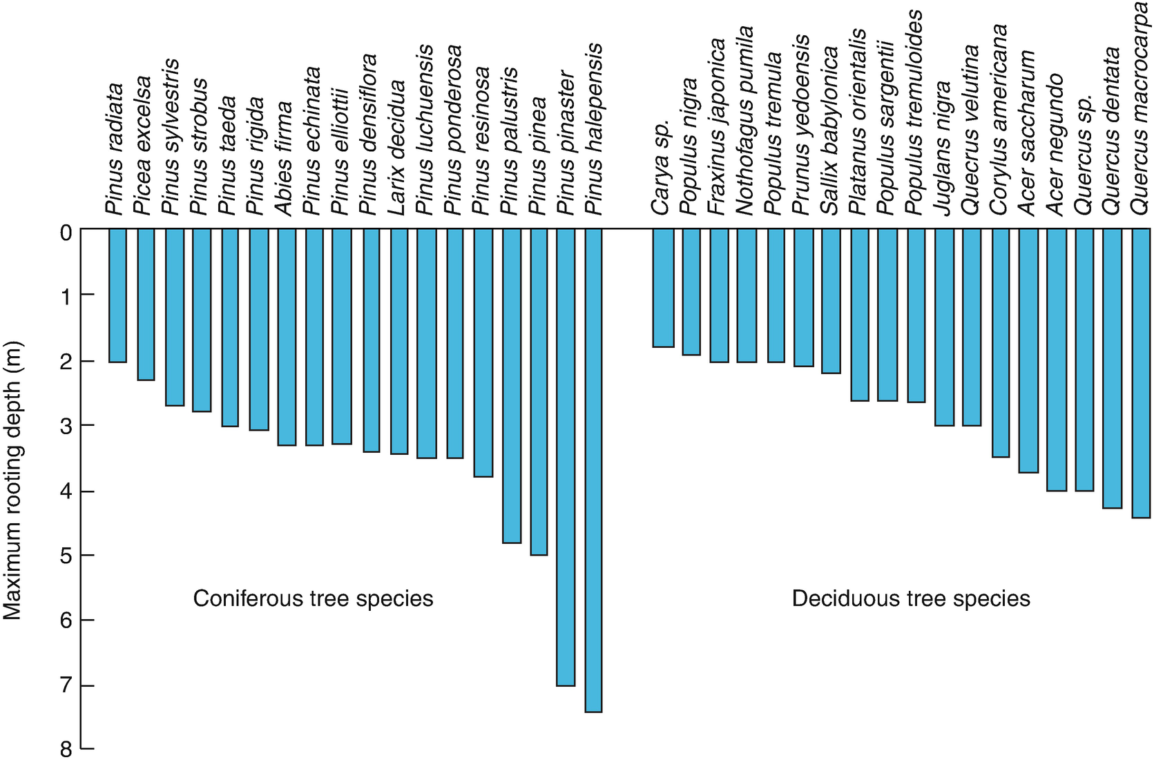
Root traits have been investigated less, but they are of course essential for water and nutrient uptake, anchoring, storage and competitive ability. Interestingly, some below-ground traits seem to covary with above-ground traits in some species, such as rooting depth and maximum height or specific root length (SRL) and SLA. However, for other species, coordination between above- and below-ground traits has not been found, which can be explained by the very different nature of the above- vs. below-ground environment and the different functions of roots, stems and leaves: roots must acquire water and nutrients from the soil solution, stems must provide mechanical strength for height growth and transport, and leaves must capture light and allow gas exchange for photosynthesis.

In addition, the presence of mycorrhizae in most plants also changes many root traits, which makes trait coordination between above- and below-ground traits even less likely (Sect. 7.​4).

Plants are immobile, meaning they cannot physically escape predators and pathogens, search for pollinators or hide from approaching extreme climatic situations. Obviously, plants as sessile organisms must continuously cope with changing environmental conditions—from minute-by-minute, daily, seasonal to decadal fluctuations in temperature and light, changes in nutrient and water availability, or herbivore pressure, pathogen load or loss of mutualistic partners. Plants have therefore evolved a variety of mechanisms that enable them to tolerate and withstand environmental change, and to re-achieve internal homeostasis: plants are highly plastic and resilient to cope with a highly dynamic environment. This phenotypic plasticity , or the capacity of a given genotype to produce different physiological or morphological phenotypes in response to different environmental conditions, is also reflected in plant traits. Traits are usually quantified comparatively across species and are highly context-dependent. This means that traits are not only genetically fixed and heritable properties, but are also plastic. They can change over time (e.g. seasonal or ontogenetic variations) and can depend on environmental conditions, the presence of competitors or herbivores and pathogens. Examples of this phenotypic plasticity of traits are the development of sun and shade leaves within a single crown (Sect. 3.​2) or the increase in defensive metabolites after herbivore attack (Sect. 8.​3). In fact, plasticity can be considered a trait of its own, given its large variability across species and habitats. Trait plasticity, however, is also limited by multiple ecological factors, for example, extreme levels in a given abiotic factor can reduce plasticity to another factor (Valladares et al. 2007).

The traits present in a plant community also reflect the interplay between evolutionary and assembly processes and the physical environment (Sect. 20.3.2). Thus, understanding how and why plant traits vary among species and sites is a critical step towards understanding ecosystem properties and their functioning. Hence, trait-based ecology has received much attention over the last decade to acquire a better understanding of how traits influence species distribution, interactions and functions (e.g. Garnier et al. 2015 for a recent synopsis with extensive literature). Global data sets covering hundreds of traits and thousands of species are available (Kattge et al. 2011), and handbooks about measurements of traits are useful for standardisation and cross-study comparisons (e.g. Pérez-Harguindeguy et al. 2013).

Once traits and their respective associations with ecological responses or effects have been clarified, different measures of functional diversity can be determined. A very critical aspect for its determination is the need to select those traits that are relevant for the process or function of interest, which thus must be defined explicitly. In general, measures of functional diversity fall into two main classes: (1) discontinuous measures, that is, categorising species into plant functional groups or types, and (2) continuous measures, that is, measuring the spread of species in an n-dimensional trait space.

20.2.3.1 Plant Functional Groups

A rather broad measure of functional richness is that of the number of plant functional groups , also often referred to as plant functional types. Plant functional types are groups of species with similar suites of co-occurring functional attributes, such as comparable physiological behaviour (e.g. C₃ and C₄ plants) (Sect. 12.​1), similar morphology or growth forms (e.g. stem succulents, lianas) (Table 20.3), temporal niches (e.g. spring geophytes, pluviotherophytes, early or late seasonal species) or similar dispersal syndromes (e.g. anemochory, zoochory) (Sect. 18.​2). In addition, functional response groups and functional effect groups are respectively species that show a similar response to a particular environmental factor (e.g. sprouters, being plants that are able to resprout after fire) (Sect. 13.​5) or that have similar effects on ecosystem processes (e.g. nitrogen fixers, which exert a significant influence on biogeochemistry). One major reason for reducing the huge variety of different organisms into such functional groups is the need to simplify floristic complexity for global vegetation models (Sect. 22.​4), for vegetation mapping, and for monitoring purposes. Methodologically, such functional groups are identified via a priori knowledge about functional attributes of species (e.g. C₃ and C₄ pathways) or by cluster analyses of trait values.

An important categorisation of functional groups in ecological and agronomic studies of grasslands is that of grasses—herbs—legumes, combining phylogenetic and above-ground architectural traits (grasses versus herbs and legumes) with physiological traits (nitrogen-fixing legumes versus non-fixing grasses and herbs). In forest ecology, the broadleaved/deciduous vs. evergreen/coniferous dichotomy is widely used. A generally applicable classification, however, is obviously not possible. Depending on the questions being posed, the same species may be classified into different groups. Many plants may belong to several functional groups; at the same time they may be “evergreen”, “zoochoric”, “deep rooting”, “nitrate storing”, and so forth, to name just a few (Fig. 20.7). Problematic is the categorisation into functional groups when considering traits with high phenotypic plasticity , because the same species may then fall into different groups, depending on the specific trait expression. Another problem with classifications into functional groups is that the ecological roles of plants are not always fully understood. It is easy to understand the function of the group Leguminosae, for example, because of its members’ ability to symbiotically fix atmospheric nitrogen, which causes disproportionate effects on ecosystem biogeochemistry (Fig. 20.8) (Sect. 16.​3), but note that the degree of N-fixation is also highly plastic and depends on soil N availability, among other factors (Sect. 7.​4). However, for groups such as “grasses” or “herbaceous plants”, this applies only partially (e.g. position of leaves and meristems, capacity to form fine roots). It is thus questionable whether such a priori subdivision of plants is justified for understanding the ecological role of species within the plant community. Classification of species according to functional groups is thus rather difficult for general purposes but might be useful for specific research questions. For example, if one is interested in whether a leaf habit in temperate mixed forests affects litter decomposition rates, the two functional groups “deciduous” versus “evergreen” tree species may already explain a large proportion of the data variability, and it may make a difference whether only one or two of these groups are present.

20.2.3.2 Continuous Indices of Functional Diversity

Much information is lost by any classification procedure because many traits are not categorical but continuous and plastic. In addition, using functional groups implies that species within those groups might be exchangeable or redundant when it comes to determining the effects of diversity on ecosystems (Sect. 20.4). Continuous measures of functional diversity , in contrast, capture the heterogeneity and variability of traits within a community. These measures can be calculated for single traits (e.g. asking the question whether the variability of leaf N concentration can better explain primary production than its mean value) or for multiple traits together (e.g. whether a higher or lower variability of leaf N concentration, cuticula thickness and LDMC better explains herbivory rates).

More than a dozen such continuous indices of functional diversity have been suggested that are based on slightly different assumptions and mathematical approaches. There are guidelines on how to select the most suitable index for specific questions (Schleuter et al. 2010; Petchey et al. 2009), and software solutions are available to calculate them (e.g. several online R scripts, FDiversity) (Pla et al. 2012). In principle, these indices can be divided into three groups that represent different aspects of functional diversity: functional richness, functional evenness and functional divergence (Fig. 20.9) (Mason et al. 2005). The first two are derived from indices to describe taxonomic diversity (Box 20.1). The latter two indices may also contain information about species’ abundances by weighting the contribution of each species based on cover or biomass, for example.

Functional richness represents the volume of the functional trait space that is occupied by the species present in a community (Fig. 20.9a, a′). It therefore reflects the potentially used niche space by a community, that is, the hypervolume of a Hutchinsonian multidimensional niche . It can be used to test the hypothesis whether ecosystem properties depend on the size of the functional space covered. For example, it could be hypothesised that a community composed of species with very different rooting depths and plant heights (i.e. high functional richness) can take up more nutrients from the entire soil profile and capture more light, and hence produce more biomass, than a community composed of flat rooting species and small statured plants only (Fig. 20.38). The index is positively correlated with species richness, but communities with the same number of species may differ in functional richness if the traits are more similar in one community than in others.

Functional evenness measures the regularity in the distribution of species abundances in the occupied trait space, with high values representing a rather regular distribution of traits (Fig. 20.9b, b′). Functional evenness can also be linked to the utilisation of resources. Staying with the aforementioned example, it could be tested whether a community with an even distribution of rooting depths and plant heights (i.e. high functional evenness) is more productive than a community dominated by flat rooting small plants because the soil profile and the above-ground space are more evenly occupied and utilised, which could lead to higher nutrient uptake and light capture.

Functional divergence estimates the position of species within the trait space, for example, by quantifying how species abundances diverge from the centre of the functional space (Fig. 20.9c, c′). A high value means that very abundant species are very far from the centre of the trait space. In our example, it can be tested whether communities with large differences in rooting depths and heights (i.e. high functional divergence) may have a high degree of niche differentiation and low competition for resources (Sect. 20.4.9), potentially resulting in increased productivity, in comparison with communities dominated by species with small differences in these two traits.

20.2.4 Phylogenetic Diversity

Next to the use of functional, trait-based indices, the quantification of phylogenetic diversity is the second approach to measuring biodiversity based on species ecological differences. The concept relies on the simple assumption that the more time that has passed since two species shared a common ancestor, the higher the probability that they have ecologically and functionally diverged. Thus, this measure of biodiversity takes evolutionary history into account. For the calculation of phylogenetic diversity, the phylogenetic trees of the organisms occurring in a community must exist, and phylogenies of many different taxa have become increasingly available in recent decades owing predominantly to genome-sequencing efforts. In principle, community phylogenetic diversity is then calculated as the sum of the phylogenetic branch lengths connecting all taxa in a community and is thus a measure of the total amount of phylogenetic distance or evolutionary divergence in a community (Fig. 20.10). Because traits are the product of evolution, phylogenetic diversity encapsulates the entire evolved trait space of a community. In consequence, it can thus be used as a surrogate for trait diversity, for example, in cases where trait information is limited (Cadotte et al. 2010).

Phylogenetic diversity is an important aspect in studying the evolutionary processes that produce patterns of biodiversity and to understand the ecological interactions that determine species assemblage (Sect. 20.3). Being a surrogate of the functional structure of communities, it is also used to test hypotheses about the relationship between plant diversity and ecosystem functioning (Sect. 20.4). In addition, it is an important measure to define conservation priorities because communities with a high phylogenetic diversity represent a larger store of genetic diversity, available for adaptation and innovation. Conserving such communities with a higher priority than those with low phylogenetic diversity would therefore maximise future evolutionary options.

20.3.1 Latitudinal Gradients

Barthlott et al. (2005) presented a detailed world map of phytodiversity (of vascular plants) that shows the large spatial gradients in plant species richness on a global scale. Such maps can be produced by overlying information about the spatial distribution of single species, which is derived from herbarium records, taxon revisions or range maps. An alternative to such a taxon-based approach is the inventory-based approach where species richness values from thousands of floras, local checklists and regional species accounts are used to calculate species richness at a specific spatial grid resolution. Since the sampled areas differ in size, the richness values for this spatial pixel have to be standardised using an empirical species–area relationship (Sect. 18.​4). Finally, non-sampled areas are interpolated using data on climate, vegetation types and geodiversity. In the map shown here (Fig. 20.11a), which uses a 100 × 100 km grid, 10 diversity zones are graded according to the number of species, from fewer than 100 to more than 5,000 per grid cell. The zones of lowest plant diversity are located in the Arctic tundra, the driest deserts (e.g. parts of the Sahara) and high alpine deserts (e.g. Tibetan upland). These regions are characterised by a lack of available ambient energy or humidity, limiting plant growth. An exception to this rule is the Namib Desert in southern Africa, which has a very long evolutionary history, high heterogeneity in topography and soils, and highly predictable rainfalls from fog in winter. The centres of highest phytodiversity are located in the humid tropics, including the Tropical East Andes, North Borneo and New Guinea, but also on the Atlantic coast of Brazil. Interestingly, not all tropical regions outnumber non-tropical ones: for instance, plant species richness in the Congo basin, where large areas are still rather undisturbed by humans, is comparable to that in Central European regions, which have been under long-term human influence. Other extra-tropical regions of high diversity are located at the Maritime Alps in France, the Caucasus or the Cape of South Africa.

Are these patterns similar for different plant life forms ? Trees, being important structural components of forest ecosystems and delivering many ecosystem goods and services, such as timber and non-timber products, are relatively well known in terms of their taxonomy and distribution. In addition, the increasing number of permanent forest inventory plots also allows for an upscaling of tree species richness to continental scales, assuming a relation between the number of species and the number of individuals of a defined region. Using standardised species lists with abundance data in such inventory plots in wet, moist and dry tropical forests, a recent study could show that the number of tropical tree species ranges between 40,000 and 53,000 in total, in contrast to only 124 tree species in temperate Europe (Slik et al. 2015)! The Neotropics and the Indo-Pacific region have very similar tree species richness (between approx. 18,600 and 24,800 species), while tropical forests of Africa are rather species poor, with only between 4,600 and 6,000 species. Thus, at least tropical trees indeed show spatial patterns similar to those shown for all vascular plants (Fig. 20.11).

So what factors are responsible for these spatial patterns? Kleidon and Mooney (2000) compared the map by Barthlott et al. (2005) with a map in which the global diversity of vascular plants was reconstructed on the basis of a climate model. Despite the different resolutions, both maps agree to a large extent (Fig. 20.11b). Obviously, climatic conditions can explain biodiversity at the global scale to a substantial degree. Climatic factors mostly constrain plant survival at the time of germination and during the development of young plants, and sufficient precipitation during those stages appears as a decisive factor: the smaller the number of days with favourable conditions for plant growth, the greater the constraints for growth and the less the diversity of species.

Also, at higher taxonomic levels, climatic factors are well correlated with diversity. Woodward (1987) found a linear relation between the number of plant families and the absolute minimum temperature (for land surfaces along a 15°N latitude). In absolutely frost-free areas, the number of plant families exceeds 250; below a minimum of 10 °C, the number is less than 100. Another, well-known example of changes in plant diversity along environmental gradients relates to the geographical distribution of tree species in North America. As shown in Fig. 20.12a, the number of tree species correlates rather negatively with increasing latitude, that is, fewer tree species are found towards the boreal zone. Climatic factors, such as mean annual temperature, annual solar radiation and precipitation, as well as actual evapotranspiration (Sects. 10.​1 and 16.​1), are positively related to tree species richness. Evapotranspiration is also strongly related to species richness of all vascular plants of North America (Fig. 20.12b). At lower latitudes between 30° and 40°N, the higher variability is also due to climatic factors: precipitation and, thus, water availability strongly decrease from east to west in this region.

But is climate indeed the only driver of global, large-scale patterns in plant diversity? What other factors might also play a role? Such questions fall within the purview of macro-ecology . Several, not mutually exclusive, hypotheses have been formulated to explain the high plant diversity in the tropics and the decrease of diversity towards higher latitudes (see overviews by, for example, Huston 1994; Rosenzweig 1995; Hillebrand 2004; Clarke and Gaston 2006). Due to lower climatic fluctuations during the ice ages in the inner tropics, long-lasting favourable climatic conditions enabled long and undisturbed adaptation and specialisation . This can be illustrated by looking at the tree diversity data: as shown earlier, Africa harbours only approx. one-fourth of the diversity found in North America or the Indo-Pacific region, which cannot be explained solely by its smaller size and lower environmental variability. Rather, African forests were shrinking to small refugia areas during the Pleistocene, resulting in large species losses. Expanding to the current area, these forests must be repopulated from a depleted species pool, while forest area in the other two regions has not experienced similar shrinkages (Slik et al. 2015). Similarly, geologically old regions of the Earth are generally particularly rich in species because of their long history of evolution compared to geologically younger parts. Higher solar radiation and higher soil water availability at the equator, leading to increased evapotranspiration, result in increased annual productivity, which is the basis for many other organisms that can exploit this resource. A comparison between global maps of net primary production (Sect. 21.​2, Fig. 21.​4) with that of plant diversity (Fig. 20.11) intuitively shows that there might be underlying factors that positively influence both productivity and diversity. This climate-driven “energy–diversity hypothesis ” has attracted substantial interest and is now considered one of the most important drivers of those latitudinal gradients (Fig. 20.12). In addition, higher predation and pathogen load all year round in tropical regions can reduce the dominance of single species, enabling the coexistence of other species with lower abundance. Finally, the tropical regions also have a higher land-to-sea ratio than regions at high latitudes, so that terrestrial diversity should be higher based on the species–area relationship (Sect. 18.​4). In contrast, climatic regions requiring specialised adaptation by organisms to harsh conditions, such as boreal forest or tundra biomes, are often relatively poor in plant species owing to strong environmental filtering (Sect. 20.3.4). For the same reasons, the number of plant species generally declines with altitude in high mountains, although the diversity in mountainous areas is higher than in lowlands if based on the available area for plant growth (Körner 2003). This has been explained by their geographical isolation and the high degree of topographic complexity and strong climatic gradients, leading to a high number of small-scale structures (habitats) in a given space, which allows many specialised species to coexist. In addition, lower human impacts and low-intensity management regimes may have led to high levels of biodiversity in mountainous areas.

20.3.2 Environmental Heterogeneity

The relation between environmental heterogeneity and species richness, as mentioned earlier in connection with alpine regions, has for a long time attracted many ecologists in the search for mechanisms driving gradients in species diversity. Almost 100 years ago, Thienemann (1920) formulated two “biocoenotic laws” stating that the more diverse the environmental conditions and the closer they correspond to the “biological optimum”, the larger the number of species, and vice versa. It has been argued that spatial environmental heterogeneity could promote species richness through three major mechanisms (Stein et al. 2014). The first mechanism is based on classical niche theory (Sect. 19.​3): the available niche space (in a Hutchinsonian sense, defined as an n-dimensional hypervolume, with the dimensions being environmental conditions, resources and biotic factors) should become larger if environmental gradients become steeper, if the amount of habitat types and the number of resources available increases, or if the physical structure of habitats becomes more complex. More species can be packed into a larger niche space.

The second mechanism is related to the ability of species to persist against adverse conditions: environmentally heterogeneous areas should provide more possibilities for shelter and refuge. This has nicely been demonstrated in topographically highly structured alpine communities. Temperature variability on the same slope of alpine grassland varies substantially at very short distances. Plant species adapted to cool habitats (Sects. 4.​2 and 9.​4), with low indicator values for temperature, grow in significantly colder micro-habitats than plants with higher indicator values found on the same slope (Fig. 20.13). Thus, species may find suitable conditions matching their thermal niche within short distances to compensate for climate warming.

As a third mechanism, evolutionary processes leading to diversification are accounted for: opportunities for isolation and divergent adaptation to diverse environmental conditions should increase with increasing environmental heterogeneity, resulting in a higher probability of speciation events. A number of studies have tested these different mechanisms and found general support of the heterogeneity–diversity hypothesis, though generalisations are difficult owing to the different research approaches, terminology and spatial scales studied. Recently, a worldwide meta-analysis that used data from 190 independent studies found general support for the environmental heterogeneity hypothesis (Stein et al. 2014). Different measures of environmental heterogeneity, including those related to land cover, vegetation diversity and structure, climate, soil variables and topography, were all positively related to species richness of plants, invertebrates and vertebrates (Fig. 20.14).

Closely related to the heterogeneity–diversity hypothesis is the intermediate disturbance hypothesis (Huston 1979), which postulates that the highest species richness will be found at intermediate levels of disturbance : at very low levels of disturbance, competitive species dominate the community and diversity is low (competitive exclusion); increasing levels of disturbance intensity or frequency may result in a disproportional mortality of the dominant species and larger environmental heterogeneity, resulting in postponed competitive exclusion, coexistence and, thus, higher diversity; very intensive disturbance events may lead to a failure of populations to recover from mortality and to a homogenisation of environmental conditions (Sects. 13.​5 and 17.​3). Thus, there should be a trade-off between the ability of a species to compete with others and their ability to tolerate disturbance. Despite being a well-recognised hypothesis, the literature shows a variety of disturbance–diversity patterns, not a consistent peak as predicted by the intermediate disturbance hypothesis (Mackey and Currie 2001). Nevertheless, disturbance is an essential feature for ecosystem dynamics and affects biodiversity to a large degree. It is a natural component in all ecosystems, working at different spatial and temporal scales. For example, soil disturbance by ants or moles creates sites free of competitors for the germination and growth of seedlings; strong crown fires eliminate dominant tree species, reducing competition for light and soil resources and allowing the establishment of other species (Fig. 20.15); ground fires destroy thick layers of litter that otherwise cannot be penetrated by seedlings and increase mineralisation of litter-sequestered nutrients (Sect. 13.​5). If such disturbances additionally act as barriers between populations, mutations that may lead to new species will have a better chance of getting established, leading to diversification over time (Sect. 17.​2), as in the Mediterranean flora of the South African Cape region or the tropical Andes, for example.

In the examples presented in the previous sections, plant diversity is statistically treated as the response variable, while abiotic and biotic site factors (e.g. availability of light, water and nutrients; disturbance regimes; herbivory) or modulators (e.g. temperature, pH) represent the independent variables that determine or explain the distribution of plant species and their diversity (Fig. 20.1). In the following section, we want to present in more detail one example of such biodiversity research, which is important to understand when we later discuss the functional importance of plant diversity (Sect. 20.4).

20.3.3 Productivity —Species Richness Relationships

There are striking biogeographical patterns of plant species diversity and several hypotheses exist to explain those patterns (Sect. 20.3.1). According to the energy–diversity hypothesis , plant diversity correlates well with measures of productivity along latitudinal gradients. Is this relationship ubiquitous and observable at various spatial scales?

Indeed, several studies have found relationships between some measures of productivity and plant species richness. It must be noted that productivity, defined as the net flux of carbon from the atmosphere into green plants per unit area and time (e.g. g m⁻² year⁻¹) is difficult to measure directly in the field (Sects. 12.​5 and 14.​1). Instead, often indirect measures that correlate to varying degrees with the potential or actual productivity of a site are used, such as actual evapotranspiration (Sects. 10.​1 and 16.​1), rainfall, peak above-ground biomass or annual biomass production. For example, in the Mongolian steppe biome, Bai et al. (2007) observed a positive linear relationship between above-ground biomass and plant species richness at various spatial scales and grazing intensities (Fig. 20.16). However, other empirical studies reported unimodal or hump-shaped relationships (also referred to as humped-back model ), with a peak of species richness at intermediate productivity levels and a decrease at very low or high productivity (Fig. 20.17). Such a decrease at high productivity—usually associated with high nutrient availability (Sect. 11.​1)—was observed in natural situations or with modified levels of productivity, for example, through fertilisation. A famous example of reduction in plant species diversity by increasing nutrient levels and associated productivity comes from the Park Grass Experiment in Rothamsted, England, where grassland plots have been treated with different fertilisers since 1859. This decrease of diversity has been compared with the paradox of enrichment of predator–prey models (i.e. that increasing availability of resources may destabilise populations, which eventually can crash) (Rosenzweig 1971). Eutrophication , via high input of fertilisers or atmospheric deposition, therefore usually leads to severe declines in plant diversity (Sect. 23.​5).

Is the hump-shaped relationship ubiquitous? A meta-analysis by Mittelbach et al. (2001) showed that for vascular plants, hump-shaped relationships indeed dominate the observed patterns, especially at local scales or in studies that crossed community boundaries, that is, that included data from several different communities. A positive linear relationship was the second most observed pattern and has been reported mostly at continental to global scales. Interestingly, several studies showed that the area below the hump-shaped relationship is often filled with data points so that the hump-shaped line may be regarded as an upper envelope curve or border line, rather than a line of fitted average values (Fig. 20.17).

What could be the underlying mechanisms producing a hump-backed productivity–diversity relationship? Several different, not mutually exclusive, mechanisms have been proposed for the increasing and decreasing part of the hump and for the peak (Fig. 20.18). In short, the hump may be the result of varying levels of resource availability and heterogeneity and of disturbance (Grime 2001). Low productivity is a result of low resource availability, as well as of low resource heterogeneity and high disturbance . These conditions allow only for small population sizes of plant species, which are therefore prone to local extinction. Only few specialised species are adapted to such conditions. Examples are the first primary successional stages, for example, in glacier forefields or rock fans (Sect. 17.​3). With increasing levels of resources and lowering levels of disturbance, more and more species are able to establish and to build up stable population sizes, and more biomass can be produced. Nutrient availability is still rather low at the increasing and plateau part of the hump, and plants mainly size-symmetrically compete for soil resources (i.e. species with larger root systems acquire more resources than those with smaller ones), which does not lead to competitive exclusion (Cahill 1999). At high levels of resource availability, coupled with low disturbance frequency and intensity, tall and highly competitive species produce closed canopies, diminishing light availability in the understorey. Competition for light is now more important than that for soil resources, and less competitive species are excluded, so diversity declines. This pre-emption of light is a good example of size-asymmetric competition for a resource of directional supply (Sect. 19.​3).

This proposed mechanism explaining the decreasing part of the hump has been supported by a somehow simple, but clever, experiment. Hautier, Niklaus and Hector (2009) assembled grassland communities in a glasshouse, fertilised them and added light to the understorey (Fig. 20.19). As expected, fertilisation increased biomass production and canopy height and decreased light levels in the understorey. In consequence, this resulted in a loss of low-statured perennial grasses and herb species. Adding light to the understorey in the fertilised plots, however, reduced competition for light and maintained plant diversity. Thus, by combining fertilisation with light addition in a full factorial design, the researchers could show that competition for light did indeed result in a loss of plant species in the face of eutrophication and related increases in productivity. From an applied perspective, this experiment gives clear arguments to prevent or reduce eutrophication owing to a surplus of fertilisers or atmospheric deposition if biodiversity is to be protected or restored, especially in nutrient-limited, species-rich ecosystems (Fig. 20.18).

Despite the fact that the humped-shaped relationship between productivity and diversity has been documented often, controversy remains about the generality of this pattern, its dependence on spatial scale, the history of community assembly, measures of productivity or other methodological inconsistencies. For example, two large-scale, global studies that applied standardised sampling designs found either general support for the humped-shaped relationship in grassland communities (Fraser et al. 2015) or no significant relationship between peak above-ground live biomass and fine-scale plant species richness (Adler et al. 2011). The differences between both studies might be due to different statistical approaches or to the inclusion/exclusion of highly productive sites, which were found to be very low in species richness, thus strongly influencing the decreasing part of the hump in the Fraser et al. (2015) study. But despite these differences, both studies showed that the humped-back model has quite low explanatory power, even if the relationship as such remains significant. Rather, it seems that productivity and richness are both influenced by a multitude of factors and processes, such as nutrient supply rates, disturbance, habitat heterogeneity, assembly history or management. Thus, instead of focusing too narrowly on bivariate patterns such as the hump-shaped curve, future investigations should look into multivariate mechanisms controlling plant diversity.

20.3.4 Biodiversity, Assembly Rules and Environmental Filters

The species composition of ecological communities is largely determined by environmental conditions, modulated by biotic interactions (Sects. 19.​3 and 19.​4) and stochastic effects, along with speciation and extinction events. Can these insights be used to predict community composition at a given location? Co-occurrence of the same species at different locations, but with similar environmental conditions, has been used in vegetation science to develop a hierarchical system of plant communities, similar to the Linnaean taxonomy of species. For example, in the system initiated by Josias Braun-Blanquet for Central Europe, vegetation is grouped according to floristic similarity into classes (e.g. European deciduous forests: Querco-Fagetea), orders (e.g. those growing on soils with good water availability: Fagetalia sylvaticae), alliances (e.g. beech and mixed beech forests: Fagion sylvaticae) and associations (e.g. those growing on poor, acidic soils: Luzulo-Fagetum). Working on North American successional trajectories, Frederick E. Clements developed the organismic concept of communities (“superorganism”), where co-occurring species are strongly linked together by interactions and a common evolutionary history (Clements 1916). This results in a deterministic development and similar final community composition at the end of successional series (monoclimax concept) (Sect. 17.​3). Among other observations, such reiterating patterns of species composition have inspired ecologists to formulate assembly rules. The concept goes back to Jared Diamond, working on bird communities on islands, who formulated empirically derived rules of community composition (Diamond 1975). This concept initiated a long and lively debate among ecologists. In principle, assembly rules aim “to specify which traits (and therefore which subset of species) will occur in a particular environment. Because the problem primarily involves traits and environments, answers should be generalizable to systems with very different taxonomic composition. In this context, the environment functions like a filter (or sieve) removing all species lacking specified combinations of traits. In this way, assembly rules are a community level analogue of natural selection” (Keddy 1992, p. 157). Environmental filters are recognised as one underlying cause of why not all species of the total species pool are actually found in a local community because of abiotic constraints, thus strongly determining the composition, structure and function of a community (Fig. 20.20). Those species that are actually absent from a community but part of the regional species pool comprise a so-called “dark diversity ” (Pärtel et al. 2011). Several factors can act as filters that lead to environmental sorting of species (Gravel 2013; Ricklefs and Schluter 1993):

• Distance of sink (local community) from source (regional species pool) and the size of the sink ecosystem. These aspects have also been integrated into the equilibrium theory of island biogeography (Sect. 18.​4)

• The structure and characteristics of the habitat (e.g. disturbance regime, nutrient status, water availability, resource heterogeneity) (Sect. 20.3)

Environmental filters thus determine the trait spectrum of communities, and certain traits determine whether a species may pass through the filter or not. Communities with a rather similar trait composition (trait convergence or trait similarity) are indicative of the presence of environmental filters because the coexisting species share ecological preferences for a specific set of environmental conditions. For example, soil fertility strongly impacts traits associated with basic physiological processes related to growth and biomass production. This “productivity filter” therefore leads to trait syndromes that reflect transitions from unproductive to productive environments (Fig. 20.23), such as those present along the leaf economics spectrum (Sect. 20.2.3). This view, also known as “weaker competitor hypothesis” (Grime 2006), states that trait convergence is the result of the competitive exclusion of species with traits associated with low competitive ability. Another example of trait convergence can be observed along gradients of environmental harshness: Communities at very unfavourable locations in terms of microclimate or soil fertility are often composed of few species that can cope with these conditions. In consequence, functional diversity decreases with increasing harshness (Fig. 20.21).

In contrast, high trait divergence (or trait dissimilarity) indicates that other ecological mechanisms are present that limit trait similarity, such as biotic filters imposed by competition. The concepts of limiting similarity and competitive exclusion and the related resource-ratio hypothesis (Sects. 17.​3 and 19.​3) state that two species that compete for the same resources—presumably due to the same trait combination—cannot coexist. That is, locally coexisting species should be functionally dissimilar to promote niche differentiation , which is one major mechanism allowing coexistence based on classical niche theory (Sect. 19.​3). Thus, other factors may still allow for coexistence, such as local disturbances that diminish the competitive dominance of few species and promote regenerative mechanisms to exploit recruitment opportunities.

The study of factors driving plant community composition, their diversity and the patterns and mechanisms of trait divergence and convergence is a lively field of research. It shows that the driving factors, such as niche-related factors, environmental conditions and their heterogeneity, change along spatial scales: at small scales, niche- and soil-related variables more strongly determine community composition, while heterogeneity and disturbance-associated parameters as well as climatic factors prevail at larger scales. In general, trait convergence or divergence depends on a variety of factors, including the selection of traits or trait combinations, the spatial scale at which environmental filtering takes place, productivity or species richness.

20.4.1 Species Identity and Dominance Effects on Ecosystem Processes

Species differ in their physical structure and biomass produced, as well as in the amounts and combinations of resources they use and in their chemical composition. Hence, different species can have largely divergent effects on ecosystem properties and processes (Sect. 19.​2). Therefore, biodiversity effects on ecosystem functioning cannot be understood without proper acknowledgement of the identity of species and their specific physiological and morphological characteristics, that is, their functional effect traits (Sect. 20.2.3). Identity effects are due to the presence/absence of particular species within mixtures and are distinct from species composition effects, which distinguish the effects of different species combinations. Examples of species identity effects are numerous. Tree species, for instance, differ widely in their effects on soil development and nutrient supply. In a replicated experiment with 14 gymnosperm and angiosperm tree species, Reich et al. (2005) observed that 30 years after the establishment of single-species plots, differences in litter calcium concentrations resulted in profound changes in soil chemistry and fertility on initially the same soils. In addition, earthworm abundance and diversity were higher in those stands where tree species rich in calcium were grown.

Interestingly, species with similar effects on ecosystem processes often coexist in plant communities, and they share similar life histories and morphological and physiological traits. This phenomenon of trait convergence (Sect. 20.3.4) can often be observed by comparing plant communities of fertile/productive and infertile/unproductive sites. On fertile sites, resource dynamics usually follow the acquisitive path of plant strategy (“fast and leaky”), with plants having high nutrient concentrations in leaves, high photosynthetic rates, high relative growth rates, and palatable and short-lived leaves with low investment in herbivore defence and that decompose fast. In contrast, unproductive sites are dominated by plants with the opposite trait characteristics and whose resource dynamics are rather retentive, that is, “slow and tight” (whole-plant fast–slow or acquisition–conservatism spectrum of plant economics, Sect. 20.2.3). Associated with such opposing trait syndromes of plants are profound differences in soil food webs and processes that are determined by the plant traits and related differences in the quality and quantity of organic matter that enters the soil (Fig. 20.23). In fertile, productive systems with acquisitive resource dynamics, litter decomposition is often mainly driven by bacteria, earthworms occur at high density, causing high bioturbation of the soil, and microarthropod density is rather low (Sect. 16.​2). As a consequence, litter decay and mineralisation rates are high, leading to high nutrient supply rates and low accumulation of necromass (i.e. dead organic matter) on the forest floor (“mull-type” humus). A lot of labile decomposition products enter the soil and are processed by microbes, resulting in high long-term stabilisation and accumulation of soil organic matter and C sequestration, especially in soils with high clay content. In infertile, unproductive systems, soil energy is mainly channelled through fungi, and soil fauna composition differs strongly from that on fertile sites. Litter decay and mineralisation are slow with low nutrient supply rates, resulting in high accumulation of necromass on the forest floor (“raw humus”). Fewer labile microbial products but more recalcitrant fungal residues will remain in the mineral soil, which also can result in the stabilisation of organic matter and high long-term accumulation of soil organic matter. Depending on the location, some of the organismic groups mentioned earlier may be absent, such as earthworms in northern North America, and their introduction will thus result in alterations of ecosystem processes, such as litter decomposition. A change of the dominance structure of a plant community, for example, due to management or changing climate, will therefore have cascading effects on soil fauna and ecosystem processes and will feed back on the plant community composition owing to the linkages between the above-ground and below-ground systems.

What is the relevance of such species identity effects for the biodiversity–ecosystem functioning relationship? Changes in land use and anthropogenic alterations of climate, nutrient cycles or consumer presence alter not only the number of species but also their relative abundance and, thus, dominance or evenness (Box 20.1). The English plant ecologist Phil Grime included the knowledge of strong identity effects in his formulation of the “mass ratio hypothesis ” (Grime 1998), which states that resource dynamics and other aggregate processes in communities and ecosystems should be strongly controlled by the structural and functional traits of the most abundant, that is, most dominant, primary producer (Sect. 20.2.3). In many cases, ecosystems are indeed dominated by one or a few species, with other species having rather low abundances (“subordinate” species) or occurring infrequently and in very low abundances (“transient” species). Hence, he argued that dominant species should have the highest impact on ecological processes such as biomass production, carbon sequestration or nutrient cycling, while subordinate species will impact these processes only to a certain degree, and transient species will have only very minor effects. Thus, the effect of dominance comprises both an effect of the degree of dominance (i.e. abundance) and the identity (i.e. presence and value of functional traits) of the dominant species. According to this hypothesis, diversity should have rather additive effects weighted by the biomass of the species present, with mixtures intermediate in performance between the corresponding monocultures. For example, Rothe and Binkley (2001) reviewed the empirical evidence on the nutritional interactions of tree species grown in monoculture and in two-species mixtures, focusing on foliar nutrition, soil nutrient supply, rates of nutrient input and patterns of root distribution. They showed that additive effects were most common, with few antagonistic and synergistic effects. Antagonistic effects are found if mixture performance is lower than expected based on monoculture performance, indicating interference competition. Correspondingly, synergistic effects could arise from positive interactions among species, such as niche partitioning and resource-use complementarity, or facilitation, for example, by nitrogen fixation of some species that increase the overall N availability for the entire plant community (Sect. 20.4.9 and Box 20.5).

20.4.2 Biodiversity Effects on Biomass Production

If single species have clear effects on ecosystems, then the next obvious question is whether adding different species to a system will result in changes in ecosystem processes and properties. In addition, it would be interesting to know whether such changes were purely additive or whether communities with more species showed some emergent properties, which can only be explained by some antagonistic or synergist interactions among species (Sect. 20.4.9). The number of studies testing the hypothesis that biodiversity affects ecosystem functioning has increased enormously in the last 20 years, so we will only be able to present a few classical and some key guiding examples. The first experiments were designed to test early hypotheses on how a change of plant species richness may affect ecosystem processes, while later experiments focused more on disentangling the underlying mechanisms of diversity effects on ecosystems. These early hypotheses (Fig. 20.24) predicted that diversity shows (1) no effect (“null hypothesis”), (2) a linear relationship between diversity and ecosystem processes, that is, loss of species causes proportional declines in ecosystem functions, or (3) an asymptotic relationship where species at higher levels of diversity might be redundant in their function (“redundancy hypothesis”). With further impoverishment of plant diversity, ecosystem functioning rapidly declines because functions cannot be maintained owing to incomplete niche occupation; very much like the loss of too many rivets leads to the failure of a machine (“rivet hypothesis” ). Species could also be primarily singular (4), and their loss or addition would have disproportionate impacts on ecosystem functioning. Cases of singular species with extreme impacts are “keystone species” or “ecosystem engineers” , with the former being species with disproportionate effects on ecosystems relative to their abundance (e.g. predators controlling dominance of other species) and the latter being species that modify the resource availability for other members of the community through modification of the habitat (e.g. dam-building beavers) (Lawton 1994). Finally, (5) the effects of species losses (or gains) might be totally dependent on the environmental context and are thus “idiosyncratic”. Interestingly, the early graphical representation of these hypotheses never showed cases, where ecosystem functions declined with increasing diversity, that is, where monocultures had higher function levels (e.g. biomass production) than mixtures. It is now clear that such negative relationships can of course also occur, and some examples are given throughout the following sections.

This overview is organised according to the scientific approaches that were adopted in the respective studies, that is, observational and experimental studies (Sects. 14.​1 and 14.​2), as well as modelling exercises. It focuses on plant species richness as the measure of biodiversity and on biomass production as an important ecological process. Effects on other ecosystem functions are presented in Sect. 20.4.3.

20.4.2.1 Observational Studies

Observational studies in natural plant communities to quantify the effects of plant diversity on ecosystem functioning can be divided into comparative studies and monitoring or sample surveys. These approaches are described in detail in Sect. 14.​1.

Here, we illustrate the use of such observational approaches with examples from forests. For instance, Baruffol et al. (2013) found in a comparative study that stand basal area (which is a measure of the area occupied by trees) and its increment over the course of 2 years (which is a proxy for stand growth) increased with the number of canopy tree species in different successional tree communities in subtropical China, even when accounting for the partial confounding of diversity and age (Fig. 20.25a). A detailed analysis of the underlying mechanisms revealed that, besides direct influences of tree diversity (which was quantified by tree species richness, functional and phylogenetic diversity), effects were driven by a combination of increased individual size of large canopy trees and increased density of smaller understorey trees at higher diversity.

Especially under a more applied aspect of timber production, a related question is whether tree diversity could also influence the stability of growth (Sect. 20.4.8). Also adopting a comparative approach, it has been shown that wood production can be more stable through time in mixed than in pure stands of very different forest types in Europe, ranging from boreal to Mediterranean forests (Fig. 20.25b). If growing in mixture, the different tree species reacted more differently to variable climatic conditions throughout the past 20 years of growth (asynchrony) and showed less temporal variation in growth through time, which resulted in overall higher stability with increasing tree species richness (Jucker et al. 2014).

National forest inventories and other permanent forest monitoring networks offer extremely data-rich and valuable tools to analyse large-scale correlations between tree species richness and ecosystem processes. Since forest inventories mainly follow silvicultural aims, some measure of tree growth prevails in those studies. A recent review showed that in nine out of ten studies, a positive association between tree species richness and biomass or wood production has been found (such as that shown in Fig. 20.26a), irrespective of forest type and biome (Scherer-Lorenzen 2014). Thus, mixtures of multiple species usually produce more biomass than the corresponding monocultures (Fig. 20.26b). However, once the confounding effects of environmental variables are accounted for, the positive diversity–productivity correlation gets weaker, and the variability of wood production explained by diversity is usually lower than that of abiotic variables, such as climate. Nevertheless, these results suggest that mixing tree species might be a silvicultural option to enhance wood production and its stability over time.

These examples show that trees growing together with many other different species are less negatively affected by interspecific competition than by intraspecific competition, presumably because of niche differentiation and resource-use complementarity , or facilitation among species, and can thus have larger growth. Such highly favourable conditions for growth in mixture may also increase resistance and resilience to perturbations or environmental fluctuations, so that trees may be able to remain productive under less optimal conditions. We will come back to these mechanisms of positive diversity effects in Sect. 20.4.9. However, there are also examples from other comparative studies that do not support these positive tree diversity effects on growth and stability and that rather suggest increased competition in mixtures than in monocultures. These contrasting views may depend on the forest type and its management; for example, silvicultural thinning to reach an optimised tree density for timber may mask any potential diversity effects on growth. Opposite patterns of the diversity–productivity relationship found in natural ecosystems may also be due to different environmental contexts, which is discussed in detail in Sect. 20.4.7. In addition, processes that favour species similarity through strong environmental filtering (e.g. harsh climatic conditions, enabling only few species with similar adaptations to persist) (Sect. 20.3.4) should result in rather low or even absent effects of plant species on ecosystem functions because diversity effects are essentially based on differences among species in functional effect traits (Sect. 20.2.3 and Fig. 20.1). However, processes that limit similarity (e.g. competition for the same resources, effects of shared pathogens) and that enable species coexistence may result in strong diversity effects, which should thus be rather frequent in natural ecosystems.

Despite these opposing views and the inherent limitations concerning causality of observed associations between diversity and function in observational studies (because both diversity and functions can be influenced by the same environmental factor) (Sect. 14.​2), there is now increasing evidence that suggests that plant species richness is an important predictor of ecosystem functioning in natural plant communities, at least in forests. The scatter in the shown data sets nicely demonstrates that additional abiotic and biotic factors influence ecosystem functions, such as climatic or soil variables, and management. In addition, identity effects are usually very prominent in observational studies, that is, ecosystem functions are often strongly determined by the dominant species (Sect. 20.4.1). Thus, ecosystem ecology and the search for biodiversity effects on ecological functions cannot be tackled as univariate problems, but a multitude of abiotic and biotic factors need to be taken into account that interact in complex ways. Another way to reduce the effects of confounding factors is the use of experimental approaches.

20.4.2.2 Experimental Studies

Experimental studies in biodiversity–ecosystem functioning research aim to decouple biodiversity from environmental conditions in order to identify causality and mechanisms of diversity effects. Thus, the level of plant diversity is manipulated experimentally by researchers. These experiments can be done in natural communities (removal experiments) or with artificially created communities (synthetic assemblage experiments or simply biodiversity experiments). These approaches are described in detail in Sect. 14.​2.

Of the two experimental approaches to studying biodiversity–functioning relations, removal experiments are highly underrepresented, although they can be useful to understand the ecosystem consequences of local, non-random extinctions, changes in natural abundance and complex interspecific interactions. For example, Wardle and Zackrisson (2005) removed plant species and entire plant functional groups from the understorey vegetation of 30 forested islands in northern Sweden. These islands differed in size, leading to a successional gradient from early successional, highly productive to late successional, less productive systems. Losses of functional groups and species decreased key ecosystem processes such as biomass production, litter decomposition and soil respiration. However, removals had strong effects on some islands but not on others, depending on island size and thus successional status and resource dynamics. This example therefore nicely highlights the importance of the specific context of study systems and shows that results cannot necessarily be generalised to other systems until properly tested.

The current thriving of functional biodiversity research and the wealth of information on the pattern of biodiversity effects as well as on their underlying mechanisms is clearly based on the use of biodiversity experiments with “synthetic assemblages”. Since environmental conditions are kept as constant as possible, disentangling diversity effects from those of the environment on ecosystem processes is possible. Several hundred such experiments have been conducted since the 1990s, and several reviews and meta-analyses have synthesised their outcomes (e.g. Cardinale et al. 2011, 2012; Tilman et al. 2014). Figure 20.27 shows results on biomass production and soil nutrient concentrations from selected grassland experiments, which can now be regarded as classical, since they spurred this field of research and also stimulated much debate about the interpretation and relevance of functional biodiversity research.

• Naeem et al. (1994, 1995) designed artificial ecosystems (“Ecotrons”) with varying species richness levels of plants, herbivores and decomposers in climate chambers. The medium- and low-diversity communities were a subset of high-diversity communities, resembling functionally depauperate descendants. Only identical species mixtures were replicated at each level of diversity. Thus, the effect of the presence of highly productive species only occurring at higher diversity levels could not be separated from richness effects. Towards the end of the experiment, high-diversity communities had lower soil nutrient concentrations and were consistently more productive than medium- and low-diversity treatments

• Tilman and colleagues conducted several large-scale experiments at Cedar Creek, Minnesota, that showed that soil nitrate concentrations within and below the rooting zone decreased with increasing numbers of plant species, while biomass production increased (Tilman et al. 1997a, 2001). Interestingly, many mixtures had higher biomass than the single best performing monoculture (“transgressive overyielding ”), refuting the sampling hypothesis as the sole explanation of the results and indicating complementarity effects (Sect. 20.4.9). On average, the diversity effects became stronger over time, due to increasing use of the available niche space (i.e. complementarity among co-occurring species). This resulted in a shift from asymptotic diversity–productivity relationships in young, developing communities to more linear relationships in mature, fully developed communities (Reich et al. 2012)

• Within the pan-European project BIODEPTH, the same basic design with manipulation of plant species richness and number of functional groups was replicated at eight different sites across Europe (Sweden to Greece). Across all sites, soil mineral nitrogen concentrations decreased with the number of functional groups (but not with plant species richness) (Spehn et al. 2005), and at the German site nitrate leaching also decreased significantly with both measures of diversity in the presence of N-fixing legumes (Scherer-Lorenzen et al. 2003). Above-ground biomass production increased with species and functional group richness (Hector et al. 1999). This effect got stronger over time and was mainly driven by complementarity, although sampling effects also contributed to the observed results. Unfortunately, not all species were grown as monocultures at some sites, which is necessary to unambiguously test for sampling effects. The biomass results also strongly differed among sites, with very large positive effects in Germany, Switzerland, Sweden, Portugal and the UK (Sheffield), unimodal or idiosyncratic relationships in Ireland and UK (Silwood) and no effects in Greece

• The Jena Experiment in Germany yielded results very similar to those described earlier: soil nutrient concentrations decreased with increasing plant species richness, or number of functional groups (grasses, small and tall herbs, and N-fixing legumes) (Oelmann et al. 2007). In parallel, biomass production increased with increasing diversity, both above and below-ground. The slopes of these relationships increased over the years, suggesting stronger and sustainable diversity effects with time. Again, complementarity effects prevailed, and the diversity-driven increase of biomass was a result of increasing plant density rather than plant size (Marquard et al. 2009)

Similar biodiversity experiments have also been established using model systems other than grasslands, including freshwater and marine ecosystems, freshwater and estuarine wetlands, intensively used agricultural systems and tundra, or tree communities. These experiments range across several magnitudes of the size of the organisms manipulated (from bacteria, algae, herbaceous plants to trees) and the size of experimental units (from glass vials, few square metre plots to 4 ha plots). In general, very similar results were obtained with such diverging systems: in more than 85% of all experiments, diversity effects on producer biomass or resource use were significantly positive, with producer biomass being 1.4 times higher in diverse mixtures than in monocultures and inorganic nutrient concentrations in soil or water being reduced by 48% relative to the monocultures (Cardinale et al. 2011). In most cases, positive diversity effects followed the redundancy hypothesis , that is, an initial loss of species has only minor impacts on ecosystem functioning because species are rather redundant in their effects on ecological processes and can replace each other. At lower diversity levels, loss of species cannot be compensated by other species. Thus, although different model ecosystems with different designs were used and the experiments were conducted by different research groups, many of the diversity–ecosystem function relationships were quite robust (Fig. 20.28).

20.4.2.3 Modelling Studies

Biodiversity–ecosystem functioning research can also be done solely on the computer, that is, in modelling studies, permitting the examination of specific mechanisms or the extension to larger spatial scales and longer time durations than empirical work. Models have been used in functional biodiversity research since early on and helped greatly in sharpening the hypotheses of underlying mechanisms. The first modelling exercises that explicitly dealt with biodiversity effects on ecosystem functioning mainly confirmed the observed positive diversity effects on productivity or nutrient retention found in experimental studies. For example, Tilman et al. (1997b) used models of interspecific competition for nutrients and randomly assembled communities with different species numbers. All species were identical, except that they differed in their R* values, that is, the concentration to which a resource is reduced by an equilibrial monoculture of that species (Sect. 17.​3 and Box 19.​2). They could show that, on average, productivity increases asymptotically with plant species richness, irrespective of the model complexity (with competition for one or two resources or with a generalised niche model). At the same time, nutrient retention also increased, which corresponds well to experimental results. This suggests lower nutrient losses at higher levels of diversity, for example, through soil nitrate leaching. In summary, the study showed that variation in species traits (R*, and the size of the niche spaced covered by each species) is sufficient to establish a positive richness–productivity relationship based on fundamental mechanisms of interspecific competition. Greater variation in species traits is magnified by interspecific interactions, which cause the average response of multispecies communities to differ from the response of the average monoculture. Both complementarity and selection effects (Sect. 20.4.9 and Fig. 20.37) contribute to this effect. Other models also confirmed the hypothesis that plant diversity can exert effects on ecosystem functions, for example, mechanistic models in spatially structured ecosystems in which plants compete for a limiting soil nutrient (Loreau 1998) or models of recruitment limitation in heterogeneous habitats or competition–colonisation trade-off models (Mouquet et al. 2002). However, these models also reveal situations where no diversity–function relationship should be expected, for instance, when species are redundant in their functional role (e.g. occupying the same spatial niche) and when the average resource-use intensity of the species is not affected by species diversity (which can hardly be found in real situations). These models also show that the slope of the diversity–function relationship depends on the mechanisms of species coexistence and on the causes of species richness gradients.

Besides the use of such models from theoretical ecology, which define species performance based on a theoretical trait space, models can also be parameterised by specific autecological traits and life-history trade-offs from real species. We present one example in more detail that nicely demonstrates how a modelling framework can be used to formulate hypotheses about mechanisms underlying diversity effects on ecosystem functioning (Fig. 20.29), which can then be tested in the field (Fig. 20.39). Using a forest succession model that was originally developed to simulate forest growth and dynamics, it has been shown that tree species richness promotes productivity in European temperate forests across a large climatic gradient (Morin et al. 2011). Interestingly, considering competition for light as the single form of species interaction and implementing real species-specific growth responses to light availability were sufficient to detect strong complementarity effects. Two underlying mechanisms could explain this, via diversity effects on mean values of forest canopy characteristics and their variability. First, higher species richness is associated with higher diversity in species traits (maximum height, growth rates, shade tolerance), leading, on average, to a higher leaf area index (LAI) of the canopy (1). Thus, functional diversity promotes light interception, which translates into higher productivity beyond that expected from monoculture performance (2). At the same time, higher light interception also means higher shading, which increases the mortality rates of smaller trees and the amount of dead biomass in the stand (3). Second, higher functional diversity in light-related traits reduces the temporal variability of LAI (4), so that incoming radiation can be better exploited, which also results in higher productivity in the model (5). Diversity also increases the heterogeneity in tree heights (and thus of light) within the canopy (6), that is, the vertical structure of the canopy is getting more complex through interspecific competition compared to intraspecific competition (monoculture). This change in structural complexity allows forests with varying traits to respond faster to small-scale mortality events, that is, they show a higher turnover in biomass (7). In sum, these main processes involved in the simulated dynamics together could explain the positive productivity response to increasing tree species richness and functional diversity.

20.4.3 Biodiversity Effects on Other Ecosystem Functions

The first experiments quantified biodiversity effects on the basis of a few ecosystem functions only—mainly measures of productivity and of resource uptake, as exemplified in the previous section. Later experiments often simultaneously measured a large variety of ecological properties and functions, including, for example, litter decomposition, carbon sequestration, soil water and nutrient dynamics, or greenhouse gas emissions. Several of these response variables are also affected by plant species composition and diversity, and some examples are presented here.

Soil physical characteristics (e.g. porosity, aggregate stability), chemical characteristics (e.g. pH, nutrient concentrations, carbon pools) and biological aspects (e.g. litter decomposition, fauna, microbial communities) (Fig. 20.30) have been found to depend on plant community composition and diversity. A large proportion of experimental work on the diversity–function relationship has been done with litter mixtures and decomposition trials, mainly owing to the rather easy possibilities for experimental manipulation of litter diversity. Several aspects of the decomposition process and the turnover of labile soil organic matter are sensitive to diversity-mediated changes in both abiotic and biotic conditions (Sect. 16.​2), including microclimatic conditions or the abundance and composition of soil fauna and microbes. In fact, there are numerous examples of mixture effects on leaf litter decomposition. In three reviews of litter decomposition studies across different vegetation types (Gartner and Cardon 2004; Hättenschwiler 2005; Hättenschwiler et al. 2005), it was shown that synergistic diversity effects are known for roughly half of all litter mixtures studied, that is, decomposition rates of litter mixtures are higher than expected based on rates of single-species litter. Purely additive effects (i.e. no biodiversity effect, meaning that the decomposition of mixed litter can be predicted by the decomposition rates of the corresponding pure litter types) are reported for a third of all cases, and antagonistic effects (i.e. slower decomposition in mixed than in pure litter) can be observed in the remaining 20% of mixtures (Box 20.5 for explanation of the terms antagonistic, synergistic and additive). The positive or negative diversity effects on litter decomposition can be direct, for example, by providing different litter qualities and quantities, or by different timing of litter inputs in highly diverse communities, which may influence litter decomposition rates. Diversity effects can also be indirect by affecting the microenvironment, for example, through different canopy closures that feed back on soil moisture and temperature, which in turn affects litter decomposition. Experimentally, such direct and indirect effects can be disentangled by deploying different kinds of litter bags, with mass loss of the litter inside the bags as a measure of decay rate: bags with a standard material (e.g. wheat straw, cotton strips) will measure biodiversity effects that are driven by changes in the microenvironment (e.g. soil moisture, temperature, humidity, UV radiation); bags with community-specific litter employed in a homogeneous, similar vegetation type, but outside the target communities (common garden approach), will measure biodiversity effects through changes in litter composition and quality; bags with community-specific litter deployed in their corresponding community will measure the combined influences of biodiversity through litter quality and through changes in the microenvironment. Under such an approach, it has been shown that litter decomposition rates increased with functional diversity of the plant community, via both such direct and indirect effects (Scherer-Lorenzen 2008).

In biodiversity experiments, soil -related functions often react with some time lag after the initiation of the experiments in comparison with those above-ground, as seen for microbial biomass, for instance (Fig. 20.30c). Most plant diversity experiments following the synthetic community approach involve some land-use change and pretreatments or soil disturbances, such as ploughing, harrowing or herbicide application, before new communities are established. Many soil organisms therefore suffer a decline in abundance. Only with ongoing succession and recolonisation by soil organisms may differences in plant community composition and diversity finally manifest in specific soil communities and functions (Eisenhauer et al. 2010; Sects. 13.​4 and 14.​2). Such findings also highlight the need to run biodiversity experiments for prolonged periods of time.

20.4.4 Biodiversity Effects on Other Trophic Levels

Changes in plant biodiversity may have cascading effects on other organismic groups and multitrophic interactions and, thus, on herbivore damage, pathogen infection, pollination success and food web structure (Sect. 19.​4). The abundance and diversity of above- and below-ground organisms, which are associated with the plant community, are often positively related to increasing plant species richness, with few exceptions (Fig. 20.31). Obviously, diversity begets diversity, at least in studies that manipulate plant diversity. In contrast, other plant species that initially do not belong to the plant community have less establishment success with an increasing number of species present. This resistance to invading species at high diversity levels can be due to lower levels of unconsumed resources left by the established species, as also predicted by resource-use models (Sect. 20.4.2), or due to fewer vacant niches. A higher degree of niche overlap between resident and invader species should also decrease invader success, and resident species having similar trait combinations (i.e. belonging to the same functional group) as invaders are often found to exert strong negative effects on invading species. In contrast, large-scale comparative studies most often find that resident species diversity is positively correlated with invader species diversity (Sect. 23.​5).The factors that determine the diversity and coexistence of resident species, such as resource supply, levels of disturbance and habitat heterogeneity, probably also influence the success of invasive species. However, the two findings are not necessarily contradictory: while the positive effect of diversity on invasion resistance operates at the neighbourhood scale, other factors that covary with diversity may be more important in determining invasion success at larger scales.

Despite such a generally positive association between plant diversity and diversity of other organisms sometimes different organismic groups have opposing responses, even within the same study, which can be explained by the degree of feeding or host specialisation, foraging patterns or movement mobility. This might become clear by looking at herbivores and pathogens that are often related to the presence of certain host species (Fig. 20.32a). Usually, generalist animal species profit from plant diversity as diets get broader, leading to higher herbivore damage in mixed plant communities. Such responses are termed—from a plant perspective—associational susceptibility . In contrast, a reduction of herbivore or pathogen damage with increasing diversity can be observed mostly for specialist animal or fungal species, a phenomenon called associational resistance . Clearly, such results are highly relevant for applied aspects, such as agriculture or forestry, where herbivores and pathogens are often seen as pests. Some meta-analyses suggest that in the majority of cases plant diversity exerts positive effects on the resistance against such pests (e.g. Jactel and Brockerhoff 2007; Castagneyrol et al. 2014), which opens the possibility of using plant biodiversity as a tool for controlling or regulating these organisms (Sect. 20.4.10).

20.4.5 Biodiversity and Multifunctionality

The quantification of many ecosystem functions within biodiversity studies opens the opportunity to quantify ecosystem multifunctionality . This term describes the fact that ecosystems simultaneously provide a multitude of ecosystem functions and services and are also often managed or valued in this respect. For example, mountain forests provide timber, protection against avalanches and landslides, continuous groundwater recharge, mushrooms and berries (so-called non-timber forest products) and recreation opportunities for hikers and mountain bikers, among other uses. It is therefore also of high practical and applied value to know whether plant diversity influences multiple ecosystem functions and services . This challenge has been tackled in several, complementary steps, and an overview of the different ways to quantify multifunctionality is presented by Byrnes et al. (2014). First, if single functions are considered that are measured at one place at one time and under one environmental change scenario (i.e. under a single setting of functional interactions or a single context), then many species, but not all, promote ecosystem functioning (Cardinale et al. 2011). Enlarging these analyses to more settings or to another context often shows that even more species are needed to ensure a certain threshold of ecosystem functioning because different species promote functioning, for example, in different years or at different places (e.g. different sites or different patches within a site) or under different global change scenarios. Second, more species are needed to provide several functions simultaneously because different species promote different functions. On average, this means that an index of multifunctionality responds positively to increasing biodiversity, as has been shown for very different terrestrial and aquatic communities (Lefcheck et al. 2015). One study combined all these different aspects and found that the proportion of species that promote ecosystem functioning increases with increasing numbers of years, places, ecosystem functions and environmental changes (Fig. 20.33) (Isbell et al. 2011). In other words, many different species are needed to maintain multiple functions at multiple times and places under changing environments, that is, biodiversity begets ecosystem multifunctionality under multiple contexts. These findings also put the concept of “redundancy ” (Sect. 20.4.2) into another perspective: although species may appear to be functionally redundant when one function is considered under one set of environmental conditions, many species are needed to ensure ecosystem functioning and the delivery of ecosystem services if multiple contexts are considered simultaneously; thus, functional redundancy is not given.

20.4.6 Different Metrics of Biodiversity Affecting Ecosystem Functioning

As exemplified by the selection of the studies discussed earlier, there is now substantial evidence that biomass production and many other ecosystem functions increase with increasing plant species richness, that is, taxonomic diversity. Does this pattern also hold true if other metrics (evenness) or facets of biodiversity (genetic, phylogenetic, functional or structural) are considered?

Increasing evenness of plant communities, that is, how evenly the abundance or biomass is distributed among species, commonly results in higher levels of biomass production. Starting with the experiments of Wilsey and Potvin (2000) in oldfields of Quebec, Canada, several studies have now confirmed their results, while others reported increased productivity with increasing dominance of species (Hillebrand et al. 2008). These contrasting results can be explained theoretically by the prevalence of species interactions influencing ecosystem processes: in the case of synergistic interactions, such as complementarity or facilitation (based on niche differentiation among species) (Sect. 20.4.9), increasing evenness should result in higher process rates, and increasing dominance to lower rates. In contrast, if species identity (i.e. the dominant trait) predetermines processes (corresponding to selection or sampling effects) (Sect. 20.4.9), these processes should be largely influenced by increasing dominance. In addition, under longer time scales with fluctuating environmental conditions, a higher evenness should allow communities to adapt to new ecological conditions and sustain ecosystem process rates due to higher trait variance. In contrast, under stable conditions, a certain optimal trait configuration should result in the highest process rates, and any deviation from this trait configuration through increasing evenness would reduce process rates.

Experiments that created a gradient of plant genetic diversity within species, for example, by planting communities with different numbers and combinations of genotypes (e.g. of seagrass (Zostera marina), wheat (Triticum aestivum), wall cress (Arabidopsis thaliana), evening primrose (Oenothera biennis) or different grassland species) also showed positive diversity–productivity relationships, often in the same magnitude as those found with species diversity (e.g. Zeller et al. 2012). Genetic diversity seems to be especially important for the temporal stability of biomass production (Prieto et al. 2015). As mechanisms, complementarity in resource use and facilitation (Sect. 20.4.9) in those mixtures of genotypes that differ in functional traits have been suggested.

Manipulating phylogenetic diversity, that is, planting communities differing in the evolutionary relatedness of the constituting species (Sect. 20.2.3), also often leads to similar results; for instance, Cadotte (2013) showed that if species were grown together with close relatives (low phylogenetic diversity) the biomass production was similar to that in monoculture. If they were grown with distantly related species (i.e. high phylogenetic diversity), they produced more biomass than expected from their monocultures. Thus, distantly related species differ more strongly in their niche requirements than closely related species, leading to an occupation of different niches that allows resource-use complementarity (Sect. 20.4.9).

Since plant functional traits may control ecological processes to a large degree, building the mechanistic bridge between species richness and its effects on ecosystems, many biodiversity experiments not only included a gradient of species richness in their design, but also one of functional diversity . In many cases, the number of functional groups (e.g. grasses, legumes, other forbs) has been varied. Quite often, but not always, such measures of functional diversity were even stronger predictors of ecosystem processes than species richness. This finding can be attributed to the fact that any diversity effect must be based on some functional differences among co-occurring species, which are better captured by measures of functional than taxonomic diversity. However, in those experiments, the gradients of species richness and of functional diversity cannot be completely orthogonal to each other (e.g. because there cannot be more functional groups than species), so that it is not possible to fully separate both factors, making the interpretation of their relative effects difficult. Building on such experiences, some newer biodiversity experiments now focus on manipulating functional trait diversity a priori while keeping species diversity constant. Including functional traits in the design may therefore allow for a better understanding of the mechanisms underlying the effects of altered biodiversity. In such approaches, a measure of functional diversity (Sect. 20.2.3) is calculated for all possible combinations of species mixtures at a given level of species richness, and the mixtures to be planted are drawn at random, resulting in a gradient from low to high functional diversity (Fig. 20.34). Alternatively, principal component analyses can be used to separate trait axes that describe gradients in trait similarity, from which mixtures differing in functional diversity can be selected. If the traits considered are related to resource-use complementarity, for instance, then mixtures with different levels of complementarity can be designed (Ebeling et al. 2014).

In analogy to the experimental manipulation of compositional or functional diversity, one might also think of biodiversity experiments that create a gradient of structural diversity , β-diversity or even landscape diversity directly, but this has not been done so far. It would be worth doing if we wish to understand the multiple effects that different facets of biodiversity may have on ecosystem multifunctionality, and across multiple spatial scales. Indeed, data from observational studies indicate that growth can be positively affected by increasing structural diversity in forest stands (Lei et al. 2009).

Although it has often been claimed that one biodiversity metric (e.g. functional diversity) should be better suited to explain diversity effects on ecosystems than others (e.g. species richness), the choice of the metric will certainly depend on the research question and on the taxa to be investigated.

20.4.7 Context Dependency of Biodiversity Effects on Ecosystems

Despite the overwhelming evidence for plant diversity effects on a multitude of ecological processes and functions, it is important to note that ecosystem functions greatly differ in their response to changes in plant diversity: some functions increase with increasing diversity, others decrease, and others hardly respond at all. In addition, the same function, say productivity, also shows divergent responses to changes in diversity in different environments or at different successional stages. Thus, biodiversity–ecosystem process relationships are highly context-dependent . In other words, the form and cause of the relationship are likely to change as the environment alters the relative contributions of species to ecological processes (Cardinale et al. 2000). This can be illustrated by comparing the slopes of these relationships under different environmental situations. In principle, two scenarios are possible, and there is evidence for both of them:

• The values of ecosystem processes could increase or decrease with changing environmental conditions, but similarly across the entire range of diversity. In statistical terms, the slope of the relation does not change, only its intercept, and the interaction term between diversity and environmental conditions will be non-significant (Fig. 20.35a). As an example, drought stress reduced biomass production at all levels of plant species richness by the same absolute value in the Jena Experiment (Vogel et al. 2012).

• The values of ecosystem processes change under different environmental conditions, but the magnitude of this change depends on plant diversity, leading to changing slopes of the diversity–function relationship, and a significant diversity by environment interaction. If the slope increases, that is, when diversity effects become stronger under a changed environment relative to a control situation, two possibilities exist (Fig. 20.35b):

  • Plant diversity effects are stronger under more favourable conditions, that is, when resources are plentiful; examples include a larger soil volume that can be exploited or higher nutrient availability after fertilisation. This biotope-space hypothesis postulates that the niche space of individual species can expand into a larger biotope space and that more species with different niche requirements can be “packed” into the niche space under more favourable conditions (Dimitrakopoulos and Schmid 2004). Therefore, resource-use complementarity can be greater and beneficial biodiversity effects should increase under favourable conditions, where high soil resource availability is hardly limiting growth. For example, diversity effects increased with fertility of the soil in an experiment with annual plant communities and NPK fertilisation (Fridley 2002).

  • Plant diversity effects are stronger under harsh environmental conditions because they often rely on facilitation or positive interactions among species (Sect. 20.4.9), which are more pronounced under harsh conditions: according to the stress-gradient hypothesis , interactions among coexisting species shift from negative (competition) to positive (facilitation) as environmental stress increases from favourable to harsh conditions (Callaway 2007). For example, in a study with freshwater marsh plants, the absolute values of biomass production decreased in more stressful environments (drought, salt, shade) relative to a control treatment, but diversity effects increased (Steudel et al. 2011). Comparative studies from natural and semi-natural ecosystems, for example, forests, mostly support the view that diversity effects become stronger under harsh conditions.

Support for both scenarios has been documented, so it is not possible to say whether diversity effects should generally be stronger under harsh or favourable conditions. Presumably, the type of environmental conditions, that is, which resources limit plant growth most, and the nature of species interactions might both be crucial for the slope of the diversity–function relationship under different ecological contexts. For example, imagine a gradient of growing conditions, ranging from low supply of soil resources, where nutrient or water availability limits plant growth, to high soil resource availability, where light is the major growth-limiting factor. If species interactions result in improved light absorption, for example, through canopy stratification, or higher light-use efficiency, then the diversity effects should be stronger under more favourable conditions, in line with the biotope-space hypothesis. In contrast, if species interactions result in greater soil resource availability, for example, through N-fixation or accelerated rates of nutrient cycling, the diversity effects should increase with decreasing growing conditions, based on the stress-gradient hypothesis. Thus, the strength of positive interactions among species (complementarity , facilitation ) will change along the gradient of growing conditions (Forrester 2014).

20.4.8 Plant Biodiversity and the Stability of Ecosystem Functioning

A long-standing hypothesis in ecology is that species diversity is positively related to ecosystem stability, which dates back to the seminal work of Charles S. Elton (1958) and which has fascinated ecologists ever since. An exhaustive overview of this “diversity-stability hypothesis” can be found in Griffin et al. (2009), Loreau and Mazancourt (2013) and Oliver et al. (2015). Interestingly, this field of ecology has been largely theory-driven. Early theory predicted that more diverse communities and food webs were more stable and more resistant to invasion by other species (e.g. MacArthur 1955). Later, Lotka-Volterra models of interspecific competition showed that communities became less stable as the number of interacting species increased (May 1973). In contrast, future statistical models showed that diversity may buffer environmental fluctuations through the scaling relationship between the mean and the variance (statistical averaging, or the so-called “portfolio effect ”), even without interactions among species (Doak et al. 1998). This portfolio effect compares the temporal stability of ecosystem functions with that of financial assets, which show lower fluctuations and, thus, higher stability when partitioned across multiple stocks. Statistical averaging can also result in a positive diversity–stability relationship in the presence of species-specific responses to changing environmental conditions and functional redundancy within groups of species (“insurance hypothesis”) (Yachi and Loreau 1999). Imagine that species differ in their requirements for abiotic or biotic environmental factors (e.g. temperature, soil moisture, nutrient availability), that is, in their fundamental niches. These species will respond to environmental fluctuations not similarly, but asynchronically, and declines in some species or populations will be compensated by increases in others, resulting in less variation in process rates at the aggregate community or ecosystem levels or in no net change of ecosystem functioning, a phenomenon called compensatory dynamics . Thus, a high diversity of species’ responses within functional groups further stabilises ecosystem functions through the asynchrony of species responses to environmental fluctuations . This mechanism can be seen as a form of temporal complementarity between coexisting species. Plant diversity can also increase the temporal stability of biomass production if mixed communities produce more biomass than monocultures (“overyielding ”) (Sect. 20.4.9) while keeping temporal variability constant.

The effects of biodiversity on stability may differ depending on the different aspects of stability. For example, temporal stability refers to a low variation of an ecosystem function over time quantified as the reciprocal of the coefficient of variation. Tree growth, for instance, is more stable over time in mixed vs. pure forest stands (Fig. 20.25). There are also many cases from experimental studies where an increase of plant species richness leads to increased temporal stability in the face of climatic fluctuations (Fig. 20.36a). Resistance describes the ability of a system to maintain its original state in the face of an external perturbation. For example, highly diverse communities are often more resistant to invading plant species (Sect. 20.4.5) or maintain ecosystem functions against climatic fluctuation (Fig. 20.36b). Finally, resilience defines the speed at which a system recovers after a perturbation (Sects. 13.​4 and 17.​4), which often is unrelated to diversity (Fig. 20.36c). These results suggest that biodiversity stabilises ecosystem functions, such as productivity, during but not after perturbations.

20.4.9 Mechanisms Underlying Biodiversity–Ecosystem Functioning Relationships

Based on hundreds of observational and experimental studies, there is now broad consensus that plant diversity affects many ecosystem properties and processes, irrespective of the metric of biodiversity used. More diverse systems consistently have higher biomass production, higher nutrient uptake and, consequently, lower leaching losses to groundwater, among other effects. What are the underlying mechanisms that could explain such biodiversity–ecosystem function relationships?

In general, trait differences among species are the underlying causes of any biodiversity effects on ecosystem functioning . In the debate about the relevance of results from manipulative experiments, often a distinction was made between the effects of species numbers and of species identities (i.e. their functional traits). Many studies have shown that the identity of species within a mixture is more important than the number of species. However, because no two species are identical in their characteristics (e.g. growth rate, size, nutrient use efficiency, leaf lifespan), it is impossible to manipulate species richness without selecting species with different characteristics. Thus, it becomes clear that there is no magic effect of numbers of species per se and that any effect will arise from functional differences between species and from species interactions. There can not be any relationship between species richness and ecosystem processes without these functional differences between species. All theoretical models of diversity–functioning relationships also include assumptions concerning differences in species’ traits, and there is no theoretical mechanism that would produce any relationship between species richness and ecosystem processes with identical species. Therefore, the characteristic traits of species and, thus, the diversity of functions these species perform are important determinants of ecosystem processes.

20.4.9.1 Sampling and Selection Effects

The sampling effect is related to the statistical chance of a species being present in a mixed community. Consider a community assembled randomly from a fixed pool of species. The probability of the presence of a species increases with increasing species richness. For example, if the pool consists of ten different species, the probability of having species A in a monoculture is 0.1. In a five-species mixture, this probability is 0.5, and it is 1.0 at the ten-species level (where species A is always present). Thus, it is more likely for that species to have been “sampled” from the pool at higher diversity. Consider further that this species has a high performance in monoculture, that is, it influences ecosystem processes to a great extent, for example, because it is a very high-yielding species or because it has high values of other functional traits. If this particular species dominates the community (i.e. “selected”), the system should—on average—tend to take the functioning imposed by that species, which is then termed selection effect (Tilman et al. 1997b; Loreau and Hector 2001). In that case, a graph showing ecosystem process rates against number of plant species will have a flat upper bound of data variation, which indicates that the ecosystem process of highly diverse mixtures is not higher than the single best monoculture. Further, the mean rate of ecosystem processes will increase as the number of species increases (e.g. increasing productivity) (Fig. 20.37a). Similarly, the level of unconsumed resources will decrease with diversity if the sampled species is able to extract soil resources very effectively. A positive selection effect therefore indicates that a species with high monoculture performance dominates the mixed-species community and its functioning, leading to a positive relationship between plant diversity and ecosystem function. The selection effect can also be negative if communities are dominated by a species with low—and not high—values of functional traits or rates of ecosystem processes in monoculture, resulting in a negative biodiversity–ecosystem function relationship. The selection effect was initially viewed as an experimental artefact, but it is a simple possible mechanism linking diversity and ecosystem functioning, which involves species interactions—leading to the dominance of one species over others.

20.4.9.2 Niche Differentiation and Resource-Use Partitioning : The Complementarity Effect

Resource-based competition theory predicts the coexistence of species if interspecific competition is lower than intraspecific competition . This could be achieved by differences in species’ requirements for abiotic or biotic resources, habitat or environmental conditions, and, hence, in their niche space. Niche differentiation allows more species to coexist, that is, it promotes diversity (Sect. 19.​3). Since plants depend on a small and common set of abiotic (water, light, CO₂, mineral nutrients) or biotic resources (pollinators, mycorrhiza, among others), partitioning of resource niches in plant communities is less obvious than in animal communities. One way in which plants could differ in resource niches is by partitioning a common resource in space (e.g. access to nutrients in different soil layers due to differences in rooting depths), time (e.g. different nutrient uptake phenology), chemical form (e.g. nitrogen nutrition via nitrate, ammonium or organic N) or a combination thereof.

Such partitioning of the available resource pool among the coexisting species allows them to use resources in a complementary way. Hence, a combination of species could obtain more resources than could any species living by itself, that is, the per capita performance of species in species-rich communities is higher than in species-poor ones. Thus, niche differentiation or resource partitioning and the resulting resource-use complementarity can lead to increased yield in mixtures compared to those of the corresponding monocultures due to a larger available total resource pool.

The principle of resource complementarity has been known for a long time. The German silviculturalist Heinrich Cotta (1763–1844) argued against large-scale afforestation with fast-growing species in monoculture, which were established on the recently developed concept of sustainability by von Carlowitz (1713): “Endeavours to establish pure stands everywhere are based on an old and highly detrimental prejudice. […] Since not all tree species utilise resources in the same manner, growth is more lively in mixed stands and neither insects nor storms can do as much damage; also, a wider range of timber will be available everywhere to satisfy different demands…” (Cotta 1828, p. 115; translation by Pretzsch 2005). He thus recognised the fact that different tree species occupy different resource niches and that this results in higher yields and even greater stability against biotic or abiotic perturbations; he also somehow anticipated the concept of ecosystem services by relating this ecological principle to human demands. Later, Charles Darwin in The Origin of Species used the term “ecological division of labour” to describe ecological niche differences that will result in higher productivity in mixed plant communities (Hector and Hooper 2002): “It has been experimentally proved that if a plot of ground be sown with one species of grass, and a similar plot be sown with several distinct genera of grasses, a greater number of plants and a greater weight of dry herbage can thus be raised” (Darwin 1872, p. 113). Since then, the concept of resource complementarity has already been successfully used for a long time in intercropping or agroforestry to increase yields per unit land area, for instance. In these cases, species with markedly distinct functional properties are chosen to produce higher yields in mixtures than in monoculture, a phenomenon known as “overyielding ”.

To illustrate this important ecological principle, consider a habitat with spatial or temporal heterogeneity of two factors that limit plant growth, such as light intensity (decreasing from the top to the bottom of a plant canopy) and soil nitrogen availability (decreasing with soil depth). Each species would occupy a certain region within this two-dimensional niche space owing to differences in plant height and rooting depth (Fig. 20.38a). It would perform best at a certain combination of light and soil N, and it would be the superior competitor with this combination. By adding more and more species (Fig. 20.38b), the heterogeneous habitat or the available niche space would be covered more completely (Fig. 20.38c). Since there would be some overlap in the fundamental niches of the species present, they would adjust their niche requirements (realised niche) to reduce niche overlap and competition (Fig. 20.38d, Box 19.​3, Hohenheimer Groundwater Experiment). At the species level, niche breadth and niche overlap between species would decrease with increasing diversity. At the community level, the niche space occupied by the species present (or total niche breadth ) and, hence, resource use would increase with species richness (Fig. 20.38e), allowing a higher biomass production. It must be noted that total niche breadth at the community level would also increase with diversity if the fundamental niches of the species did not overlap at all, that is, the effect would be purely additive and without the need to adjust the niche space with coexisting species. If different, randomly chosen species combinations are present at each level of species richness in a mathematical model, the resulting graph would thus show an asymptotic increase of mean total community biomass with increasing species richness until the resource pool is used up completely (Fig. 20.37b). The upper bound of the data cloud would also increase, indicating that some mixtures perform better than the monocultures, which cannot be explained by selection effects but only by complementarity or positive interactions among species in mixture. Hence, spatial, temporal or chemical resource complementarity has been suggested as an important mechanism underlying the often observed positive relationship between plant diversity and productivity or nutrient cycling. These different forms of complementarity are not mutually exclusive but can occur simultaneously in a mixed community.

Typical examples of resource-use complementarity are mixtures of small and large statured plants, of plants with shallow and deep roots, of sun-adapted trees in the overstorey and shade-tolerant species in the understorey, of early successional and late successional species, of warm-season and cold-season grasses, or of nitrate- vs. ammonium-preferring species. In agroforestry and intercropping, such species have also been called species with good “ecological combining abilities” because they face less competition in combination with other species than when growing only with conspecific neighbours.

Box 20.5: Distinguishing Between Selection and Complementarity Effects

Discussions about the interpretation of early biodiversity experiments mainly centred on the question whether the observed patterns could be explained by niche complementarity or by the selection effect. It is now clear that these two classes of mechanisms are not mutually exclusive and that they can occur simultaneously. In addition, in most experiments, selection effects prevail during the early phases owing to the exponential growth of species that develop quickly and dominate mixed plots initially. Later in the course of the experiment, competitive dynamics take over and niche complementarity effects become stronger (Reich et al. 2012).

But how can one distinguish between these two classes of mechanisms? First, the visual inspection of the diversity–functioning patterns and their upper bounds can indicate the prevalence of selection or complementarity effects if all species are present at all diversity levels (flat in the case of selection effects, increasing in the case of complementarity effects, Fig. 20.37a, b respectively). However, since both complementarity and selection effects can produce similar patterns in a graphical representation and because both effects can occur at the same time, the underlying mechanisms cannot be inferred from patterns alone. Thus, mathematical approaches have been developed that are based on comparisons of plant community performance (e.g. biomass production, nutrient uptake) in monoculture and in mixtures. A very often used method is the additive partitioning approach, developed by Loreau and Hector (2001), which is a further development of approaches used in agronomic studies that calculate the relative yield (RY) of a species, that is, the yield of a species in mixture related to its yield in monoculture, and the relative yield total (RYT) of the entire community. The additive partitioning method calculates a net biodiversity effect (NE) and partitions it into two additive constituents: the complementarity effect (CE) and the selection effect (SE), with NE = CE + SE. If biomass production (or yield) is used as a response variable, the net effect is the difference between observed yield in mixture and the average of the monoculture yields, with a value NE = 0 being indicative of equal growth of plants in mixture and in monoculture (“additive” effect) (Fig. 20.39). The complementarity effect is the difference between observed relative yields (i.e. yield of a species in mixture expressed as a proportion of its yield in monoculture) and the expected relative yield (i.e. null-expectation values or the proportion of the species seeded or planted in mixture). Values of CE > 0 indicate positive or “synergistic” biodiversity effects by resource complementarity or facilitation , while CE < 0 indicates “antagonistic” effects due to competition by physical or chemical interference. The selection effect occurs when relative yields of species in mixture are related to their monoculture biomass, calculated with a covariance function. NE, CE and SE are usually expressed in dimensions of yield but can be adapted to any ecosystem property measurable at the species level. As shown in several single studies and meta-analyses, NE and CE increase with increasing numbers of plant species and with time, while SE usually fluctuates around zero in most biodiversity experiments, which indicates that niche differences and positive interactions mainly drive biodiversity effects on ecosystems (e.g. Cardinale et al. 2007).

Mathematical approaches are helpful to detect complementarity effects and to distinguish them from selection effects (Box 20.5), but they do not indicate a specific biological process responsible for the observed effects. Thus, other approaches are needed to obtain a more mechanistic understanding of the role of plant diversity in ecosystems. For instance, below-ground resource complementarity can be quantified by determining the species-specific root distribution within the soil or by injecting nutrient or water tracers (e.g. distinct isotopes of nitrogen or water) at different soil depths, at different times of the year or in different chemical forms and measuring their uptake by plants. Above-ground, niche differentiation and complementarity for light can be related to the surface of light-absorbing tissues (mainly LAI) and community light capture (light attenuation within the canopy) or to detailed measures of canopy packing or space filling. Values of the LAI and other measures of plant canopy complexity often increase with increasing diversity, as well as with densities of the vertical stand profiles and community heights, all being indicative of higher canopy packing. Optimised canopy packing, which fills the available space more completely with photosynthetic active tissue in both space and time (e.g. through phenological niche differentiation), can thus be an important mechanism of above-ground resource complementarity to increase total light interception and canopy photosynthesis.

The role of complementary architectural traits in optimising canopy packing of mixed communities and the relevance of vertical stratification and crown plasticity can be illustrated nicely with tree stands, where the individual crown dimension can be rather easily quantified (Fig. 20.40). Vertical stratification occurs if tree species with different crown architectures and adaptations to shade coexist, thereby displaying leaves in distinct height strata. Such multilayered canopies develop, for example, during succession, when shade-tolerant, late successional species regenerate and grow under the canopy of light-demanding pioneer species. Crown architecture is additionally highly plastic, as trees adjust their height growth and branching patterns in response to neighbours: alteration of light intensity and of red/far red ratios , that is, light quality, will result in shade-avoidance reactions such as increased height growth (Sect. 3.​2).

For example, using a network of 209 permanent forest plots across Europe, spreading a gradient of tree species richness at each of six sites, Jucker et al. (2015) were able to show that canopy packing increased significantly with the number of tree species within a stand. This positive diversity–canopy packing relationship was partly driven by differences in vertical crown stratification between different species (i.e. by mixing species with different canopy heights) (Fig. 20.40b). In addition, species increased crown volume (i.e. developing longer lateral branches and deeper crowns) in mixture compared to monocultures (+38%), thereby showing phenotypic plasticity in response to hetero-specific neighbours (Fig. 20.40c).

Increased canopy packing by mixing species will enhance light interception, may increase litter production and alter microclimatic conditions and offers higher structural complexity. These changes will further affect productivity, biogeochemical fluxes and the diversity of other organisms. Thus, managing forests with the goal of safeguarding these functions may be achieved by increasing canopy packing and its structural complexity through mixing of tree species. However, there might be trade-offs between different management goals. For example, increased canopy packing may offer more structural heterogeneity and, thus, more habitats for canopy-living organisms, such as insects or birds (Fig. 20.6). But it may also result in higher light absorption in the tree canopy, and thus lower light availability at the forest floor for understorey vegetation, as well as cooler and dryer soil conditions that also negatively affect nutrient cycling. This highlights the need for local, site-specific management decisions, which might include a weighted valuation of different ecosystem functions or services (e.g. higher value for birds than for understorey plants) or which might include additional silvicultural interventions (e.g. reducing stand density to allow greater light penetration to the understorey).

20.4.10 Value of Biodiversity–Ecosystem Functioning Research

After almost two decades of intensive research, biodiversity–ecosystem functioning science has come into a phase of synthesis, fostered by several reviews (Kinzig et al. 2002; Loreau et al. 2002; Naeem et al. 2009; Weisser and Siemann 2004; Scherer-Lorenzen et al. 2005; Hooper et al. 2005; Tilman et al. 2014) and meta-analyses (Balvanera et al. 2006; Cardinale et al. 2006, 2007, 2011). The insights gained are all highly relevant for our fundamental understanding of how ecosystems work and how plant diversity controls ecosystem processes. However, how reliable are results from biodiversity–ecosystem functioning research, which is still largely based on some “artificial” experimental manipulation? Are biodiversity experiments suitable to predict the consequences of species changes in real ecosystems? Can the results from biodiversity–ecosystem functioning studies guide us in developing effective nature conservation or ecosystem management strategies? Can we design sustainable production systems based on the insights obtained from knowledge of biodiversity–ecosystem functioning? Especially for experimental approaches, these questions have generated controversy, despite the fact that they focus on general patterns and ecological mechanisms and less on applied problems of nature conservation (for an overview, see Duffy 2009).

20.4.10.2 Relevance of Biodiversity–Ecosystem Function Research for Sustainable Production Systems, Nature Conservation and Ecosystem Management

Based on the assumption that diversity effects are generally robust (and there is now substantial evidence for it, at least from experiments directly manipulating diversity), we can suggest that biodiversity can be used as a tool to enhance productivity, stability and other ecosystem functions in production systems while at the same time reducing the input of agrochemicals and fertilisers. Starting from performance and trait expression in monocultures, it is possible to design optimal species combinations for the delivery of single or multiple ecosystem functions or services (e.g. Storkey et al. 2015). However, it must be taken into account that performance may change in mixtures owing to phenotypic plasticity, which will also lead to different observed levels of ecosystem function in mixtures than what would be expected based on monoculture performance (Sect. 20.4.9). In fact, there are several examples showing that high-diversity mixtures of plant species utilised in intensively used grasslands, forests or bioenergy production systems produce equivalent or sometimes even greater quantities of biomass than monoculture-based systems (e.g. Dickson and Gross 2015; Finn et al. 2013), often at lower levels of herbivory and inputs of fertilisers or other agrochemicals and with lower losses of nutrients or trace gases. Such low-input, high-diversity systems may thus be a sustainable option for biomass production, such as for forage, biofuels or biomaterials, which can combine conservation and greenhouse gas mitigation goals with production orientated goals (Tilman et al. 2006; Weigelt et al. 2009). Such production systems should have substantial advantages over high-input, low-diversity systems, especially in conditions of high environmental heterogeneity , as illustrated in Fig. 20.41. The upper solid curve shows the diversity–yield relationship under conditions of low environmental variability, for example, constrained by high fertiliser and pesticide input or irrigation. In this case, a single, very highly productive species grown in monoculture can achieve yields higher than or comparable to those of polycultures (blue dots). Farmers and foresters have selected such high-yielding or fast-growing species to maximise yields in short time spans, supporting them by excluding competing species or adding soil resources. Examples include corn (Zea mays), switchgrass (Panicum virgatum), Douglas fir (Pseudotsuga menziesii) or eucalypts (Eucalyptus spp.). In contrast, the lower dashed line shows the same relationship under conditions of large spatial or temporal environmental heterogeneity, for example, where it is too costly or impossible to homogenise the environment via agrochemicals, fertilisers or irrigation. In that case, polycultures of complementary species (due to niche differentiation) will produce higher yields than single species.

Finally, it can be questioned whether changes in biodiversity can have effects comparable to those of other drivers of global change , such as eutrophication , climate change or land-use change , which have significant impacts on ecosystems (Chap. 23). At least for biomass production, there is accumulating evidence that the effects of species loss are on the same order of magnitude as those of eutrophication in the form of nitrogen deposition or nutrient fertilisation, drought stress, fire, herbivory or elevated CO₂ (Hooper et al. 2012; Tilman et al. 2012). Thus, the global loss of biodiversity we are facing today is certainly one of the major drivers of changes in ecosystem functioning and, thus, is also strongly affecting the delivery of ecosystem services for humanity. Hence, besides ethical considerations, the strong control that biodiversity has on ecosystem multifunctionality and stability should be another, utilitarian argument for conservation and restoration of biological diversity in the era of human dominance of almost all global ecosystems.

Nevertheless, we close this chapter with a note of caution: high biodiversity or high levels of ecosystem functioning are often a reasonable goal for nature conservation or ecosystem management , but they are not always “good” or “desired”: for example, an increase of plant diversity in naturally species-poor ecosystems, such as raised bogs, is often indicative of substantial changes in site conditions, for example, through drainage. Similarly, an increase in productivity in oligotrophic ecosystems, such as acidic grasslands, is also often due to human-induced changes in resource availability, for example, through fertilisation or atmospheric nitrogen deposition. We should therefore base conservation efforts not only on general biodiversity–ecosystem functioning relationships, but on ecosystem- and site-specific targets of biodiversity (e.g. rare species, keystone and umbrella species, representative communities, natural seral communities) and ecological processes (e.g. predator–prey interactions, pollination, soil stabilisation, carbon sequestration).