
The species-rich segetal flora in an annual crop of lentils and in a perennial crop of olive trees demonstrates the typical anthropogenic replacement of communities in an area of the European Mediterranean region that is still little influenced by herbicides. (Photo: K. Müller-Hohenstein)
17.1 Introduction
The historical development of plants and of plant communities is discussed in Chapter 17. Plant communities develop over the course of time and may display directed or cyclic dynamics. Their history of development must be known to understand their actual structure. In the geological epochs up to the Holocene, plants and plant communities developed in close connection with numerous climatic changes. Only in the Anthropocene did the influences of human activities start to take on growing importance. Today the loss of plant species and the spread of neophytes are the main forces of change.
17.2 Development of Plants during Life History on Earth
-
Continuous migration of the continents in relation to the poles. According to measurements of palaeomagnetism, the magnetic North Pole in the Cambrian was in the Pacific, not far from the current location of the Japanese island group, whereas it was in north-eastern Asia in the Triassic (Fig. 17.1).
-
The formation of continents arising from the permanent changes in the position of parts of the Earth’s crust (continental shift and plate tectonics) (Fig. 17.2).
-
Solar effects (different radiation conditions) arising from the composition of the atmosphere, coupled with changes in the Earth’s eccentricity (orbit) around the Sun.
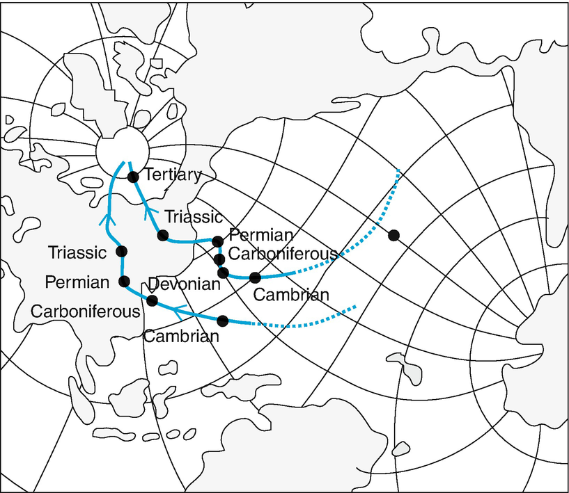
Changes in position of magnetic North Pole during geological time, determined from palaeomagnetic measurements of North American (upper curve) and British rocks (lower curve). (after Kreeb 1983)

Stages in development of present distribution of continents. a Joined landmass of Pangaea in Triassic. b Distribution of continents at end of Cretaceous. (after Bick 1993)
These events are linked to two influences directly affecting plants and their evolution. Firstly, climatic conditions have changed drastically and, secondly, the possibility for area expansion of plants and animals by the opening or closing of land bridges or by the rise of mountain barriers was either limited or enhanced. Furthermore, catastrophic asteroid impacts as well as changes in the CO2 levels (Sun et al. 2012) that greatly reduced biodiversity at the end of the Permian and the Mesozoic should be mentioned.
More recently, the development of the patterns and distributions of vegetation has changed worldwide more rapidly and to a much greater extent by the continuously growing influence of human settlement and changes of land use. This shows clearly that palaeo-ecological links and historical development must be known to acquire a better understanding of present-day vegetation and its structure, composition and spatial distribution.
In the following section, periods of the history of life on Earth, including selected aspects of the phylogeny and coevolution of organisms (eophyticum, palaeophyticum, mesophyticum), will be outlined. The Neophyticum will be discussed in more detail, with special emphasis on late and postglacial development of vegetation, as well as direct and indirect influences of humans on plant cover. Problems of global change will be discussed more comprehensively in Chap. 21.
17.2.1 History of Vegetation to the End of the Tertiary
In the Precambrian Period two large separate landmasses existed, each near the poles: the Laurasia continent in the Northern Hemisphere, and the Gondwana continent in the Southern Hemisphere. These two continents over time merged and became the continent of Pangaea. Pangea remained one mass until the Palaeozoic Period, where changes in positions towards the poles and equator occurred. Traces of life and the first single-celled prokaryotes (bacteria, cyanobacteria) existed for about three billion years in an oxygen-poor atmosphere. Eukaryotes and multicellular forms could only develop when increases in oxygen occurred in the environment. This period, extending into the Silurian, is called the eophytic (proterophytic) or algal period.
An important plant developmental step occurred during the Silurian Period, where colonisation of land happened from the eophytic to the palaeophytic period. The first land plants possessed cells with large vacuoles, and some were able to develop stomata and other supporting tissues. These autotrophic plants lived together with fungi and bacteria (primary decomposers) communities and formed the first biocoenoses. From that period, plant diversity continuously increased through evolution.
Putative evolution of life forms and ecosystems during Earth’s history (after Kreeb 1983)
|
Time in millions of years |
Geological formation |
Plant |
Animal |
Ecosystem type |
|
|---|---|---|---|---|---|
|
Neophyticum (angiosperm period) |
0 |
Present |
Agricultural techniques |
Homo faber |
Anthropogenic ecosystem disruption |
|
0.005 |
Holocene |
Cultivated plants |
Domestication of animals |
Anthropogenic changes in ecosystems |
|
|
0.5 |
Pleistocene |
Homo sapiens |
All land ecosystems, deserts, halophytic communities, cold areas |
||
|
30 |
Tertiary |
Deciduous trees |
Freshwater fish, humanisation |
||
|
95 |
Cretaceous |
Angiosperms |
|||
|
Mesophyticum (gymnosperm period) |
150 |
Jurassic |
Pine trees, first flowering and seed plants |
Early birds |
Plant adaptation to different climate zones |
|
200 |
Triassic |
Dinosaurs, early mammals |
|||
|
Palaeophyticum (pteridophyte period) |
230 |
Permian |
Species diversity decreases slightly |
||
|
280 |
Carboniferous |
First tree-like ferns: Lycopods Calamites Horsetails Ferns |
Reptiles and dinosaurs |
Swamp forests (dry land not colonised) |
|
|
340 |
Devonian |
Lung fish, amphibians, insects |
First highly developed land ecosystems in moist places |
||
|
450 |
Silurian |
First land plants: early ferns |
First vertebrates |
Simple ecosystems without consumers on land near coasts |
|
|
Eophyticum (algae period) |
500 |
Cambrian |
Algae |
All animal types except vertebrates |
Higher developed aquatic ecosystems |
|
2000 |
Algoncium |
Photosynthesis, respiration using oxygen |
(Oxygen atmosphere) simple aquatic ecosystems |
||
|
3000 |
Archaean |
First chemosynthetically active organisms |
(Anaerobic aquatic ecosystems?) thermophilic organisms |
||
|
4000 |
Early ocean/early atmosphere |
Start of biological evolution: first cells |
(Oxygen-free environment) (salt-free ocean?) |
||

Age and development of important groups of vascular plants and of phyto- and entomophageous insects. First occurrence of insect pollination and herbivory is also shown. (after Zwölfer 1978)
During the transition from the Carboniferous to the Permian Period, climatic conditions became much dryer. Many species became maladapted, which led to extinctions as many plant species were unable to adjust their water retention capabilities. Thus, the transition from the palaeophytic to the mesophytic is highlighted by a significant decrease in plant diversity. Colossal shifts in landmasses occurred at the beginning of the Triassic, when the Tethys Ocean separated from the eastern part of Pangaea. During the Jurassic, the North Atlantic developed, while the southern Atlantic formed during the Cretaceous Period. In the early Tertiary Period, Antarctica and Australia broke off as well, and it took up until the Pliocene to arrive at the present position of the continents we see today.
Up to the Cretaceous Period, global flora was generally similar in diversity. The oceans at this point were still too small to be considered barriers to the exchange of flora. The history of vegetation up to the mesophytic is also called the period of the gymnosperms. Following the extinction of the larger club mosses and horsetails, gymnosperms, particularly conifers, were able to expand their distributions. In the northern regions the first representatives of the Pinaceae and the genus Juniperus are found. Cupressaceae occurred worldwide. The boundary between the Jurassic and Cretaceous Periods also divides the mesophytic from the neophytic and the gymnosperms from the angiosperms. The first angiosperms occurred at the end of the Jurassic Period.
In 25 million years of the Cretaceous Period, flowering plants developed rapidly and outcompeted many of the gymnosperms, which up until then had dominated. Almost at a snap of the finger all the main angiosperm groups developed, and all suitable habitats were colonised. Intercontinental flora exchange was still possible and helped facilitate the rapid rates of colonisation. A stronger floristic separation occurred during the Upper Cretaceous Period. The so-called plant kingdoms developed and created the three floristic realms in the Southern Hemisphere, Antarktis, Australis and Capensis, two tropical equatorial floristic realms, Neotropics and Palaeotropics, and the Holarctic, the sole Northern Hemisphere floristic realm.
Zwölfer (1978) gave the first overview of geological occurrences of vascular plants as well as phytophageous and entomophageous insects, which addressed the development of communities. It was reported that both pollen and dead plant material were eaten by arthropods as early as the Devonian Period, and in the Permian leaves were consumed. In the Triassic, insect pollination of flowers occurred, and there were entomophageous parasites and plant galls. From the Tertiary onwards, all present-day phytophages are represented: miners, gall flies and gall gnats (Fig. 17.3).
Mutual adaptations of floristic and faunistic partners (vertebrates as well as invertebrates) result when selective pressures are linked in development. Plants developed thorns, spines or chemical defence substances, whereas animals adapted through changes in their mouth parts or developing resistance against plant toxins. Some flowering plants were able to protect themselves against herbivory, for example, Gentianaceae (defence by indoalkaloids) or Solanaceae (defence by tropanalkaloids); however, again this led to the development in some animals of an ability to adapt to some of the most powerful plant toxins. In some cases animals made use of these substances for their own defence (Sect. 19.4, Chap. 19).
Most groups of flowering plants were present at the beginning of the Tertiary Period. The neophytic or angiosperm period is the current period. Among flowering plants, specialists are resilient in the most stressful environmental conditions (e.g. desert, highly saline soils, bare rocks). Along with the formation of mountain ranges, young mountain floras developed (oreophytes, sometimes closely related to flora in plains). Often individual altitudinal steps are characterised by vicariad species and genera. An example of altitudinal vicariation in the Alps is Anthoxanthum odoratum for grasslands at lower altitudes and Anthoxanthum alpinum at higher ones. Another example of ecological vicariation is the alpine Rhododendron species R. ferrugineum, which grows on siliceous rock, and R. hirsutum, which grows at the same altitude but on calcareous rock.
Holarctic flora has been found in Palaeozoic to Eocene lignite deposits in Spitsbergen, where not only the remains of plants growing in today’s Central Europe under conditions of a temperate climate were found (e.g. Acer, Betula, Fagus, Quercus, Pinus and Picea) but also those that now grow only in humid, subtropical regions (e.g. Taxodium, Magnolia, Liriodendron). Plants found in Greenland represent the so-called arcto-tertiary flora, the basis of the Holarctic flora (e.g. Aesculus, Castanea, Platanus, Vitis). From the Eocene “flora from the Geiseltal” near Merseburg, Germany, plant lists were compiled containing tropical plant families (e.g. families Annonaceae, Pandanaceae, Sterculiaceae). The question thus arises as to how tropical genera can grow in areas currently characterised by cold-temperate climatic conditions. Plate tectonics is the justifiable answer, where Europe had only taken up its current position in the Northern Hemisphere during the Tertiary Period.
In plant remains found from the Pliocene in Central Europe, tropical species are absent, but present-day genera (Fagus, Quercus) indicate a worldwide progressive cooling. In Europe, climate and vegetation zones shifted to the south. The development of new barriers began to become an issue, where the west–east extension of the Alps and the Mediterranean Sea made it difficult for certain species adapted to a warm climate to survive, where some species went extinct and others were able to survive in local refuges or simply migrated to more favourable regions. The relative uniformity of Pliocene flora in the Holarctic was lost. Large distribution ranges were separated into several spatially limited regions, the large Tertiary disjunctions (different separated parts of the former area of distribution, e.g. Sequoia and Metasequoia). For other species, for example, of the genera Styrax, Platanus, Melia and Castanea, a few moist warm sites became important refuges. The development of Mediterranean sclerophyllic vegetation is often connected to the general cooling of global climate in the Tertiary Period. Cooling in the Pliocene may be regarded as a precursor of the multiple quaternary climate changes, especially when compared with those occurring in the Pleistocene and Holocene.
17.2.2 Change of Climate and Vegetation in Pleistocene
The change from warm to cold periods is very important for the development of the vegetation in Central Europe. Temperatures continued to decrease in the Pleistocene for about two million years, which periodically would change to brief cold (“ice ages”) and warm periods. Average annual temperatures decreased here by at least 8 °C and as much as 12 °C below present-day temperatures. These climatic variations in the early Holocene are mainly explained by periodic changes of solar radiation caused by alterations in the orbit of the rotational axis of the Earth.
Direct and indirect consequences of Quaternary climate variations may be summarised as follows: On both hemispheres, starting from the polar regions, enormous inland ice masses up to 3000 m thick developed. Massive alpine glaciers also were present in the higher mountainous ranges. During the glacial maximum, few peaks rose beyond the alpine ice cover (nunataks). The glaciers extended far north into the foothills of mountainous regions, where a mere 300 km of ice-free area between alpine and polar ice caps in Europe remained. At the same time, sea level sank to about 200 m below the present level (eustatic changes) so that movement of plants in the cold period became easier between landmasses currently separated by shelf oceans (e.g. land connection between England and the European continent).
-
Biber and Danube ice age in the early Pleistocene about one million years ago;
-
Günz and Mindel ice age in the middle Pleistocene, about 250,000 years ago;
-
Riss ice age about 230,000–120,000 years before the present (BP);
-
Würm glaciation (about 90,000–12,000 years BP) in the late Pleistocene.
The extinction of warmth-requiring tropical and subtropical species became more extensive, as did the alternating dominance of woody species during the warm periods and herbaceous species and grasses during cold ones. Trees in particular disappeared locally or survived unfavourable periods in refuges of eastern and southern latitudes. Because herbaceous plants, grasses and low-growing dwarf shrubs expand at much faster rates owing to their shorter regeneration times, this also resulted in far fewer losses of such species. Some thermophilic species were able to occupy refuges and survived, but their original continuous distribution was eventually separated into several disjunct areas. One of these disjunct distributions has cedars, with some species in the North African mountains (Cedrus atlantica), in the Near East (Cedrus libani) and in the Himalayas (Cedrus deodora).
During cold periods, very few species (mainly mosses, lichens and high alpine flowering plants) successfully inhabited mountainous regions surrounded by glaciers on the nunataks. The southern range expansion of some species has also been attributed to the changing climate during cold periods. There are several migratory paths, for example, the East African Rift Valley, the American mountain ranges and the bridge in South-East Asia-New Guinea-Australia, where these plants found places to grow and even today occur in bipolar distribution regions. Examples are the genera Carex, Erica, Epilobium and Empetrum.

Distribution of vegetation types in Europe during time of maximal glaciation in Würm glacial period. (after Kreeb 1983)
17.2.3 Late and Postglacial Climate and Vegetation History
-
The enormous evolution of species and plant communities dependent on astronomic, tectonic and climatic events in biocoenoses.
-
A distinct spatial separation of large parts of the Earth’s crust occurred, with orogenesis reaching the actual situation.
Now, in smaller areas, changes of the floristic characteristics due to small-scale differences in the site conditions are more important. Following the Holocene Period, the continents had almost reached their current position. The result was an irregular pattern with approximately 71% of the globe covered by water and the remaining 29% constituting continental land masses. The latter are unequally distributed with a large maximum in the Northern Hemisphere. Furthermore, large mountain ranges formed in Eurasia, extending mainly from west to east and north to south in the Americas. These main features have a determinant role in regional, continental and global climate, and, thus, impact the distribution and dynamics of vegetation.
Because of the outstanding example of the north–south extension of the Cordilleras, the different atmospheric conditions in the Americas, coupled with the regional pattern of glaciers and ice sheets, together form a developmental process different from what has occurred in Europe. Plant migration following the climatic changes was easier because difficult-to-cross west–east barriers like the European alpine mountain chains are missing. We concentrate here on the development in Eurasia and Africa.
|
1000 |
XII |
Forest plantations Beech |
Postglacial |
|||
|
Post-interglacial period (sub-Atlanticum) (relatively cool and moist) |
Historical period |
|||||
|
0 |
XI |
Iron Age |
||||
|
−1000 |
X |
Beech-oak |
Late interglacial period (Sub-Boreal) (warm and dry) |
Bronze Age |
||
|
−3000 |
IX |
Mixed oak forest (oak, elm, lime, ash) |
Late |
|||
|
Middle interglacial period (Atlanticum) (warm and moist, climate optimum) |
Middle |
Neolithic |
||||
|
−4000 |
VIII |
|||||
|
−5000 |
Early |
|||||
|
−6000 |
VII |
Hazel |
Early interglacial (boreal) (warm and dry) |
Mesolithic |
||
|
−7000 |
VI |
Hazel-pine |
||||
|
−8000 |
V |
Birch-pine |
Pre-interglacial (increasing temperatures) |
|||
|
IV |
Tree-poor tundra |
Late subarctic period (return of cold) |
Late Ice Age |
|||
|
−9000 |
III |
Birch-pine |
Middle subarctic period (Allerod) (temporarily warmer) |
|||
|
−10000 |
Palaeolithic |
|||||
|
II |
Tree-poor tundra |
Early subarctic period |
||||
|
−11000 |
1 |
Treeless tundra |
Late arctic period (cold) |
Main glaciation |
||
|
−12000 |
||||||

Development of altitudinal zones of vegetation in northern Swiss Alps since maximum of Würm glaciation. (after Strasburger and Sitte 1998)
and lake levels can be taken. Furthermore, changes in orbital axes and solar radiation can also be used to draw inferences from the patterns and the likelihood of the presence of certain species in the past. Finally, for the last few centuries anthropogenic greenhouse gases and remarkable land cover changes have contributed directly or indirectly to more recent vegetation changes.
On the basis of the various sources of data, some models have been developed and have proposed findings that suggest detailed accounts of climate fluctuations leading to reactions of plant communities. Controversy still surrounds the causality of these findings, which continue to be discussed (Gallimore et al. 2005; Holzhauser et al. 2005). The difficulty in attributing the causes to one factor or a number of factors lies in the fact that there are many aspects that contribute in combination with a high order of complexity in terms of the processes and how they can change with climate. The differences are often due to the different data included in modelling that have been considered as decisive (e.g. atmosphere–ocean–land data, glacier or lake-level changes, solar activities or albedo changes).
So far, the results allow two general interpretations. The first involves researchers seeing a possibility or a necessity to put the results in a system of periods. This method has been traditionally done in pollen analysis, which was built from the diagrams of Firbas (1952 ff) and Overbeck (1975) and later improved by Holzhauser et al. (2005) and Joerin et al. (2006). The second interpretation involves incorporating variability in an attempt to discern general trends, for example, cooling or warming, under humid or arid conditions (Prentice and Jolly 2000; Wanner et al. 2008).
-
Late- and postglacial times and early Holocene (18,000–9000 BP).
-
Mid-Holocene (9000–6000 BP).
-
Late-Holocene and preindustrial time (6000 BP–1700 AD).
In these three phases the development of the vegetation is closely connected with climatic changes. The influences of the late Holocene, where a remarkable human aspect begins to be identified on the vegetation, will be dealt with in the next subchapter.
In the late glacial period, also called the Dryas Period after the indicator species Dryas octopetala, a continental steppe dominated by scattered tree-free tundra islands was reconstructed after the results of pollen and macrofossil vegetation relics. All over the Northern Hemisphere, the cold, dry conditions led to different tundra and grassland types. Forest biomes were displaced southward, the boreal (i.e. taiga) biome became largely fragmented, while at the same time the moist tropical and temperate forests saw significant reductions. It is argued that during this period the arid Saharan mountains we know today may have been linked with the Mediterranean and tropical forest biomes and may have led to some of the discontinuous or fragmented range disjunctions, for example, Acacia spp. and Euphorbia balsamifera (Deil and Müller-Hohenstein 1984).
A noticeable warming of the climate occurred around 12,000 BP and was accompanied by the retreat of alpine and continental glaciers. As a result of this retreat of the glaciers, many species filled the newly created void of space. Warm-demanding species, in particular trees, were able to take advantage of this space in Central Europe. In Northern Europe, the forest biomes extended into the present-day tundras, while in the South, large parts of the Sahara were invaded by tropical grassland and dry shrubland.

Pollen diagram from Luttersee. The lake is situated near Göttingen, northern Germany, 160 m a.s.l.). Scale: sum of tree pollen 100%, without hazel (Corylus). (after Walter 1986)

Undisturbed and disturbed raised bogs. a Part of the almost natural “Pillermoor” (1600 m a.s.l.), which is a protected area in the lower Pitztal (Tyrol, Austria). b Part of same raised bog where peat was removed more than 30 years ago. Pollen analysis from this bog shows the postglacial development of vegetation of the montane region in Tyrol. (Photos: K. Müller-Hohenstein)
During the following 6000 years, the temperatures remained high with a number of distinct fluctuations. Consequently, the vegetation cover also changed; in the warmest periods (e.g. Alleröd period, Atlantic period), sparse spruce and birch forests and willow shrubs were able to exist. The steppes advanced from the east under the still extremely continental conditions. The temperate forest was able to extend; birch was methodically replaced by hazel and other deciduous trees. Human populations in the Mesolithic (about 8000 BP) were surrounded by species-rich forest communities. Remnants of tundra occupied the increasingly melting edges of the continental ice sheet, and steppes were pushed by invading forests towards the south and south-east.
This development is also confirmed by results of tree-line studies. The position of the alpine tree line in the last 12,000 years was approximately 1200 m lower in the last glacial period compared with present day conditions, outlined by the remarkable warming over this period (Fig. 17.5). The variation of the tree line, as well as a recently published temperature reconstruction, outlines similar temperature fluctuations following this temperature increase in the middle-late glacial period (Marcott et al. 2013). Throughout the early Holocene the temperatures stayed—with some regional variations—at this level. In the European Alps the tree line was about 400 m higher than today.
The warmest climatic conditions, and the corresponding development of vegetation, were experienced by the early Neolithic people in the Atlantic period about 6000–7000 BP. In Northern Europe, during this time of the “climatic optimum”, mean annual temperatures were 2–3 K higher than present temperatures. Mixed oak forests with deciduous trees requiring warm climatic and nutrient-rich edaphic conditions were dominant. In the montane areas, fir dominated in the western Alps, spruce in the eastern Alps and pines in the eastern part of Central Europe on nutrient-poor sites. Thermophilic species still occurred at dry sites with grassland vegetation.
Glacial relicts from the cold periods are still maintained in present-day vegetation in isolated sites, for example, Betula nana in the foothills of the Alps in peat bogs. Similarly, species from the warmest periods were also able to persist on limestone outcrops. These xerotherm relicts, sub-Mediterranean species (Quercus pubescens) and those from the south Siberian and Pontic areas (Stipa spp.) were able to survive after the onset of cooling in the Sub-Boreal forest. To ensure their survival, both of these relict species required specific microclimatic or edaphic conditions. For xerotherm species, extremely shallow and southern facing, exposed sites, which inhibit the growth of trees, are needed. Beech only became dominant in the forests of Central Europe in the Atlantic period and took over the role of hornbeam (Carpinus betulus), which dominated in the interglacial period and was now predominant further to the east. Together with spruce and fir, beech forms forests up to the montane belt. Even though beech has dominated the forests of Central Europe for only a relatively short time period (30–50 tree generations), beech-dominated forests became established everywhere, up until increased human intervention became more intense (Hasel and Schwartz 2006).
-
a continuous decline in temperatures and.
-
growing human influence (Sect. 17.2.4).
The climatic cooling (between 0.1 and 0.3 K over 1000 years) was the most important reason for large-scale plant migrations. Species that required higher temperatures migrated back into warmer regions and outcompeted the cold-period vegetation, except for a few relict species. Their expansion partly followed the edges of the ice sheet, and thus many closed areas became divided, and disjunctions were formed. Some of these disjunctions are concentrated on the Southern European mountains (e.g. species of the genera Primula and Saxifraga), while others form the arcto-alpine disjunctions with interspersed occurrence on the highest parts of the mountains of central Germany (e.g. Nigritella nigra agg.). Supplemental examples of disjunction distributions include the Betula nana and Salix herbacea and the circumpolar Loiseleuria procumbens and Eriophorum scheuchzeri in North America.
A reconstruction of the changes in global temperatures shows a constant decline in temperature, which ended only in the nineteenth century (Marcott et al. 2013). Especially thanks to a comprehensive palaeo Vegetation Mapping Project (BIOME 6000; Prentice and Jolly 2000), our knowledge about vegetation development from the mid-Holocene on has been considerably deepened. The reconstruction of the vegetation cover was made possible through the use of extensive pollen and macrofossil records. Vegetation was classified on the basis of plant functional types (PFTs), biomes, and mega-biomes with worldwide contributions to this programme (Harrison and Prentice 2003). Because of high summer insolation and warmer temperatures, plant species with high heat demand experience very advantageous conditions. Therefore, the vegetation distribution compared to present-day conditions, and not including anthropogenic influences, has led to a significant northward shifting of boreal and temperate species in the Northern Hemisphere. Although variability exists and depends on the region, all distributions were more than 100 km further north compared to today. Warmer winter temperatures also favoured a change from cold-temperate mixed forests to temperate deciduous forests. The Mediterranean subtropics, however, were covered with temperate grassland and xerophytic shrubland.
Only in recent decades have new data been collected in connection with the history and climate of the arid African areas (Holzhauser et al. 2005; Knorr and Schnitzler 2006). According to these findings, the long-established views of a synchronous sequence of cold and warm periods in higher latitudes (e.g. Central Europe) and dry and humid ones in lower latitudes (e.g. Northern Africa) must be corrected.

Rock paintings and engravings indicate once more humid climatic conditions in central Saharan mountains. Pictures of hunters a and large grazing herds b near Sefar (Tassili), southern Algeria, are nearly 8000 years old. The “crying cows from Terarart” c near Djanet are about 5000 years old and indicate a gradual increase in aridity. (Photos: K. Müller-Hohenstein)
There is sufficient evidence from glacier- and lake-level studies in the Swiss Alps with high-resolution data that natural driving forces still contribute to climate change (Holzhauser et al. 2005). Also, the results of tree-line studies from Russia underline a continuous cooling, at least more or less synchronous for the continents of the Northern Hemisphere (MacDonald et al. 2000a, b). Only in the last 300 years, despite the input of volcanic aerosols and a certain variability in solar insolation (both of which initiate cooling effects), has it been exceeded by the warming effect of the input of excessive greenhouse gases and land-use changes (shifting of forest to agricultural lands), which has ultimately led to a reverse forcing of the biophysical drivers for the continuous cooling seen in many regions. The main driving force for all these changes in the vegetation cover is no longer exclusively a change in climate; we must now consider anthropogenic effects in all biomes.
17.2.4 Changes in Vegetation Owing to Human Influence
Human activities have always affected vegetation because humans are directly or indirectly dependent on plants for raw materials, food and feed for agricultural livestock. The influence of humans historically was fairly small and restricted to simple consumption for themselves and their livestock. However, over time, with the rapid growth in population sizes, coupled with advances in technology and our use and the distribution of plants across the world, that influence has changed dramatically. The mosaic of anthropogenic plant communities became more diversified, corresponding to the type, duration, intensity and extent of human influence. Gathering beneficial wild plants for food and medicine, wood cutting, grazing and especially hunting and clearing, assisted by fire, led to specific “substitute communities”. Soon, coppiced forests, managed meadows and other previously unknown plant communities arose. An important contribution to the diversification of human-made vegetation types brought the lessons learnt from hunting and gathering to all agricultural activities to improve plant cultivation and animal husbandry (Box 17.1).
Box 17.1: Typical Methods of Forest and Agricultural Management
A. Forestry

Coppice with standard system (“Mittelwald”): This is a form of forest management applied in the Middle Ages (Fig. 17.9c) in combination with agriculture. The best individual trees (primarily oak) were harvested to supply timber for construction (“standards”), while the remaining trees were selected via coppicing. This technique is still used today to harvest valuable oak for veneers. Thus, an open canopy of uneven aged trees was consistently maintained to provide a sustainable supply of timber for use in construction.
High forest system (“Hochwald”): This consists of trees that grew from seeds (in contrast to regrowth from coppiced trees) (Fig. 17.9b). High forest systems are the dominant forest management strategy today. There are different varieties of this system: (1) clear-felling (clear-cut), where all trees within a cutting block are cut at the same time; (2) shelter-wood felling, where a portion of the canopy trees are harvested, while the remaining portion provides canopy protection for the understorey and seed production and are typically distributed uniformly over the harvesting block. This management strategy leads to uneven aged stands, where successful regeneration in the European systems consists of beech, coming through the understorey, while pine and oak are harvested in the overstorey. As a result, canopy trees can be twice as old as the mean stand age. For example, oak becomes most valuable for timber beyond 300 years, where the space between individual trunks is filled with some younger tree generations in order to minimise the growth of shoots from dormant buds; (3) selective cutting and gap felling, whose tree harvests result in stands that are not of uniform age; only some of the trees are removed according to their size and usefulness. Regeneration in selectively thinned forests takes place where the individual trees have been removed. Because of variations of light and size in the regeneration area, a species-rich and multi-storey forest results.
ARD: Afforestation, reforestation and deforestation attained particular significance in the onset of the Kyoto Protocol (Chap. 21). Deforestation refers to harvesting an entire forest and converting the area into other uses (e.g. roads, agriculture), reforestation is re-establishing areas of forest that had previously been forested but changed to another land use (e.g. planting of forests in valley meadows), and afforestation means the establishment of forests on land that had not been forested earlier (e.g. forests on moorlands). Revegetation is the re-establishment of forests on areas that had been free of vegetation (e.g. slag heaps). Degradation is the result of harvesting of wood in excess of its natural growth, self-thinning and the density it would reach had the stand attained maximal growth. The current definition of a forest (10–30% cover, 2–4 m high) allows degradation of these limiting values before conversion (e.g. from primary to secondary forest or to plantations).
B. Agriculture
Managed grasslands: This term refers to meadows and swards that used in the production of hay or silage or for grazing. In Central Europe, these grasslands occur mainly on heavier (clay) soils, which are difficult to plough in spring, or in areas where the growing period is too short for cereals (mountain meadows). The species richness of this strategy depends on the intensity with which they are used (e.g. frequency of cutting, fertilisation).
Arable farming: Distinctions based on the following criteria are made (Swift and Anderson 1993):
Type of soil manipulation: ploughing, disc-harrowing. With the latter, a breakdown of organic matter in the soil is reduced and seed is sown in the furrows made by the disc harrow. This method decreases the compaction of soils and leads to deeper rooting, which may increase yields in semi-arid regions. There is no soil manipulation with zero tillage.
Type of crop: root crops (potatoes, beet) and cereals. Earlier agriculture employed intensive soil manipulation and thinning after sowing as a means of controlling weeds and crop density. Today, hoeing is less essential as weeds are controlled chemically and the number of crop plants is technically regulated by sowing density. In cereal cultivation, a distinction is made between winter cereals, sown in the autumn months, and spring cereals, sown in spring. Spring cereals have smaller yields, but they avoid the risk of frost damage in winter. Particular types of crops are those grown for oil seed (rape: sown in autumn; sunflower: sown in spring) and maize, which is sown in late spring after frost (typically in May) because it requires warm temperatures for growth. Cultivation of oil seeds and maize in Central Europe has increased considerably in recent decades. Also, crops for bioenergy have growing importance (e.g. straw from cereals).

Typical types of agricultural land use in countries around the Mediterranean. a Subsistence farming in a small area with mixed crops and many cultivated plant species (Central Atlas, Morocco). b Grain crops and fodder plants for national market on large-scale farms with high input of agrochemicals and machinery (Tuscan Hills, Italy). c Mixed agroforestry with grain crops for grower consumption and cork (Quercus suber) for national market (Extremadura, Spain). d Unregulated, excessive grazing with severely degraded forests and soil erosion (Central Atlas, Morocco). (Photos: K. Müller-Hohenstein)

Typical processes and sequences in exploitation of tropical rainforest. Examples from Central Sulawesi, Indonesia. a Uncontrolled clearing (slash and burn) of primary forest, done often by groups of people without knowledge of methods appropriate for the environment. b Agricultural use of the cleared forests for only a few years (without fertiliser application) until the fertility of the land is exhausted by the cultivated plants grown to fulfil people’s needs. c The unproductive area is abandoned and quickly invaded by alang-alang grass (Imperata cylindrica) and bracken (Pteridium aquilinum). (Photos: K. Müller-Hohenstein)
Agroforestry (predominantly in the tropics) describes management systems in which forest regeneration and timber production (for fodder and fire wood respectively) are linked to field crop production in space and time. The overstorey is used for timber production, while field crops are grown in the understorey. Species of both strata are deliberately selected to optimise resource complementarity, which results in higher yields.

Types of sustainable agricultural land use in the humid as well as in seasonally moist tropical regions, across all continents. a “Continuous” rice cultivation in South-East Asia often combined with cultivation of different palm trees (Sulawesi, Indonesia). b In almost all tropical regions, small home gardens are multi-storied with different layers of cultivated plants, which “copies” the species-rich tropical forests, for example, trees such as oil palm (Elaeis guineensis), cashew nut (Anacardium occidentale) and banana (Musa paradisiaca) and annual vegetables below (Guinea-Bissau). c Sophisticated irrigation schemes on widespread terrace complexes have been in use for many centuries for cultivation of annual crops such as sorghum (Sorghum bicolor) and perennial shrubs such as coffee (Coffea arabica) and qat (Catha edulis) in the Yemen Arab Republic. (Photos: K. Müller-Hohenstein)
The present-day global distribution of vegetation can only be understood in light of human-induced influence and its associated effects on the plant community for the past few millennia. Nowadays, in Central Europe, no plant communities exist that have not been influenced by humans. In the absence of humans, it would be easy to have a vast closed cover forest across the entire European continent, for the exception of the area above the tree lines in the high mountains. At least in Europe and East Asia, the present vegetation is the result of interactions between the requirements of humans in different cultural situations and resources that offered natural landscapes. Most of these interventions are linked to the development of sedentary agricultural societies in Central America and—especially important for Europe—in East Asia.
17.2.4.1 Early Land-Use Influences
The area surrounding the Bay of Bengal, the northern Savanna landscapes of India, the Yangtze region of China and the highlands of Mexico are some of the oldest centres of agriculture (von Wissmann 1957). There is now proof that these agricultural centres had access to a number of different agricultural techniques since at least 14,000 years (Bar-Yosef 1998). Agriculturalists are thought to have come from the Levant about a thousand years later, where they arrived via Iran in Mesopotamia and essentially replaced the hunter-gatherers already located there (Hillman et al. 2001). The first technical advance was irrigation.
From this region of the Fertile Crescent agriculture and animal husbandry (cultivation) reached Central Europe via the Mediterranean region. The important steps in the shift away from a culture based on pure hunting-gathering to one that developed through the use of many techniques to improve crop growth had already taken place outside Europe. Neolithic agriculture in southern-central Europe has been found to have started about 7000 years ago, while the northern region began roughly 5500 years ago, generally limited to areas with the best climatic and edaphic conditions (dry, warm, but often nutrient-poor sites) as present in sparse mixed oak forests.
17.2.4.2 Land-Use Influences from Neolithic to Middle Ages
For a long time the effect of prehistoric man on the cover of vegetation was severely underestimated. Today, it is possible to prove the effect of these human activities for the periods in which, during postglacial times, the edges of the ice sheet retreated and woodland species immigrated. Agricultural activities (clearing and burning) contributed already during late-Neolithic times to the excessive release of greenhouse gases (GHGs) in the atmosphere and leading to human-induced climate warming. Furthermore, the intensified rice cultivation in Asia has consistently contributed to GHG emissions, where significant levels of methane are a primary by-product (Kerr 2013). Deforestation, soil erosion, nutrient depletion of soils, and land-use changes have led to often irreversible impacts worldwide, especially since the industrialisation of many larger countries over the past 300 years.
In the Neolithic Age, “unregulated forest-field management” was the most important type of land use in Central Europe. After clearing, agriculture was practised for a few years. Then the area was left fallow for a long period. Regulated rotation with sowing, grazing and use of wood in certain restricted periods in an area was only developed in the Bronze and Iron Ages (about 3700 BP), when sickles and iron ploughs replaced the wooden hook plough. The major crops grown during this period were primarily wheat, emmer and spelt. At the regional level, buckwheat was important, as were barley and rye later. The primary livestock of cattle and pigs were used to graze in forests, where the canopy trees provided wood for housing and firewood.
The first coppiced forests were developed in the Bronze Age. Wood was used for charcoal kilns and the smelting of iron ore. Hedges grew along species-rich edges of forests and nutrient-poor meadows, and dwarf shrub heathland expanded, leaving the regeneration of grazed forest areas endangered. Many deciduous trees were harvested for their branches (lopping) to provide livestock food for the winter. Thus, natural vegetation was not only considerably changed on arable fields and replaced by crop plants and their accompanying vegetation, but also in structure and species composition. In addition, large areas around settlements were influenced by grazing, trampling and tree felling and the use of other non-timber forest products, such as leaf litter.
For the last 2000 years, the youngest history of climate and vegetation development has been the focus of IGBP’s “Past Global Change” (PAGES 2k) project (Kaufman et al. 2013). A continued cooling event has been confirmed with modest fluctuations (Little Ice Age between 1550 and 1850, with three warmer intervals) until the beginning of the industrial period (circa 1700 AD). During this period, on average, global temperature was still 0.3 K lower than that found over the last millennium. These findings should be taken with a grain of salt, as considerable variability and a combination of anthropogenic and natural drivers skew the effects at the local scale.
In Central Europe, until the beginning of modern times, human activity focused on clearing areas for agricultural purposes and settlements. Forests were degraded by grazing animals and by the increasing demand for wood, which was the sole energy source for cooking and heat prior to the use of coal. The ratio of forest to open land at the end of the first clearing period was approximately 70:30, despite Neolithic and Roman settlements. In the thirteenth century this ratio flipped to 30:70. Natural forests were restricted to areas unfavourable for agriculture. Not only was the vegetation cover changed drastically, but considerable soil erosion also occurred, outlined by the alluvial deposits in most European valleys (Dotterweich 2008). Towards the end of the Middle Ages, considerable breakdowns within the social system would lead to slight increases in forested areas. At the dawn of the sixteenth century, some of the first forest regulations were enacted as a means of protecting and limiting the use of forests. As early as the twelfth century, in some regions, the grazing of goats in forests was already forbidden.
The remaining forests were structurally and floristically changed. To maintain the energy requirements and to consciously save areas of forests for grazing, coppiced forests were managed. Oak and hornbeam were particularly suited to this kind of forest management because they regenerate easily through coppicing. The fruits of oak, beech and hazel were not only important feed for livestock but were also consumed by humans. These species were thus cultivated in open forests so shade-demanding woody species decreased. Oaks were grown not only for acorns (animal feed) but also for their bark, which was used for tanning. Large, emergent trees were retained as standards in the coppice system for timber, which was required for construction (Box 17.1A).
Forest management strategies like that of the “thinned coppice” allows several light-demanding herbaceous and woody plants to become established. However, losses of species can occur owing to heavy grazing from livestock, in addition to the use of leaf litter and humus-rich topsoil for barns. The excessive collection of humus and leaf litter contributed significantly to the loss of nutrients in the system and led to large differences in fertility between forests and arable land. Excessive use of forests on sandy soils caused the formation of heathland in Northern Europe. Chronicles describe the scarcity of wood, which led to the use of peat from bogs.

Human influences on the vegetation of Central Europe. Including harvested timber and fodder yields, as well as estimates of timber reserves and soil erosion. (after Ellenberg 2009)

Development of a central European river valley landscape. Increasing deforestation, drainage, erosion and deposition of loam in flood meadows in upper and lower reaches of river. 1 Beech forest; 2 oaks and other mixed deciduous forests; 3 alder swamp; 4 conifer reforestation; 5 willow scrub; 6 other scrub; 7 wet grassland; 8 moist grassland; 9 dry grassland; 10 arable fields; 11 loess soils; 12 meadow loam; 13 moorland; 14 gravel; 15 other soil types; 16 mean groundwater level; 17 highest water level. (after Ellenberg 2009)

17.2.4.3 Agriculture and Forestry in Industrial Times
Since the onset of the Industrial Revolution and continued urban sprawl, significant changes have occurred in plant communities, where even the smallest of areas have now been affected (Sukopp and Wittig 1998). In the past, localised ploughing, watering and draining had an effect that was only apparent at a specific scale; however, as the influence of supplying and managing resources and their waste products increases, so does the effect on living systems. Pollutants and the effects of fertilisation have undoubtably influenced vegetation. For example, atmospheric deposition of nitrogen currently exceeds natural background levels by three orders of magnitude in some regions, leading to a steadily increasing eutrophication of terrestrial ecosystems (Galloway et al. 2004).
The beginning of the industrial period is linked with new anthropogenic influences on plant cover. At the onset of industrialisation, most of the remaining forests of Central Europe had already been degraded and the soils were much eroded or depleted of nutrients, which left the upper layers acidified. Although the conditions of the forest were maintained, the change in dominant energy source (coal) led to a significant makeover in terms of people thought about forest management. As the use of coal began to increase, many traditional forestry practices were no longer used; however, the demand for timber, paper and energy grew with the onset of the steam engine and railway.

Important human-made forest types in Central Europe and North Africa. a Almost naturally mixed forests (Quercus faginea, Q. rotundifolia, Cedrus atlantica) with trees of all age classes in central Atlas Mountains (Morocco). b Beech forest close to Bayreuth (Bavaria). Trees are clear felled or the largest trees are selectively removed. c Oak forest (Quercus robur, Q. pubescens) in Burgundy. The best stems for timber are only felled after 100 or more years, the rest for firewood every 30 years. d A Eucalyptus coppice in northern Morocco, cut 2 years before with new shoots forming that will be harvested after 12–15 years. (Photos: K. Müller-Hohenstein)
Managing the forest using these strategies was successful for many reasons: forests were no longer used for livestock grazing, pruning or sod-cutting, and the use of leaf litter was significantly reduced, which in turn returned substantial amounts of nutrients back to the system. The most important change in these forests was the change from the once dominant deciduous trees to conifers, which triggered a change in vegetation dynamics. All coniferous species, particularly pine and spruce, are relatively undemanding in terms of regeneration and can be sown without major drawbacks. Furthermore, conifers tend to grow quite rapidly, resulting in much shorter rotational periods (80 years) than those of oak, which can be twice as long. The extent of this change from predominantly deciduous forests to coniferous forests is considerable, as depicted on maps of German forests over the last few centuries (Fig. 17.9).
Reforestation with only conifers can cause significant problems for forest communities. Soil erosion and acidification are higher in spruce plantations than in mixed deciduous forests. Bird diversity is also significantly reduced, where the number of species and their abundance is half as much in conifer stands as in deciduous forests (Goudie 1994). These findings were reinforced in the Chilean deciduous forest, where differences were more abrupt compared with exotic pine plantations (Finckh 1995). It is well known that coniferous plantations typically have much less food resources for birds and also lack the multi-tiered structures found in deciduous-dominated stands.
The separation of forest use and grazing was also important for the development of vegetation in open spaces. To protect forests and arable land from animals, fences were put around grazing areas. In early summer with a surplus of food, animals tend to favour the most palatable species. Areas of eutrophication due to the excrement deposits of livestock and grazing areas gave rise to a characteristic pattern. Particularly noticeable was the damage caused by trampling and erosion by too many animals. This can be counteracted to some extent through the use of mineral fertilisers, and changing the variety of crops can improve yields. Soils of low fertility were fertilised and sown with grass (Vergrünlandung). Meadows were mowed, often several times per year, to provide enough fodder for animals that were kept in stables during the winter months. Cereal fields were also used for grazing after harvests, which affected segetal flora. Nutrient-poor meadows were invaded by scrub, and sites for thermophilic and xerophilic species became rarer. These examples show how new agricultural techniques and trade patterns affected the composition of plant communities.

Characteristic grassland communities in Central Europe according to water and carbonate availability. (modified from Schreiber (1995))
Already 20 years ago, Vitousek et al. (1997) estimated that between one-third and a half of all terrestrial ecosystems had been transformed by human activities, more than half of the total surface of freshwater resources is used by humans, and one-quarter of the bird species on Earth have already gone extinct as a result of anthropogenic influences. More recently, Ellis et al. (2010) characterised the artificial changes in the terrestrial biosphere since the Industrial Revolution on the basis of gridded global data for human population density and land use. According to their evaluation of the past three centuries, the terrestrial biosphere passed from mainly “wild” to mainly “anthropogenic”. With fewer small subsistence farms it is no longer necessary to combine arable crops with animal husbandry. The former “balance” of forest, grazing land and arable land once required in the rural landscape for reasons of greater self-sufficiency has now been lost. The impacts of human transformation of ecosystems over such a short time span during the last few decades has no parallel in the past with respect to intensity and consequences. Nowadays, even more drastic and irreversible shifts of global ecosystems are being discussed, potentially threatening Earth’s ability to sustain humans and other species in the near future (Barnosky et al. 2012).
17.2.4.4 Recent Developments in Forests, Arable Fields and Settlements
Intensifying production in agriculture continues apace. Machines in agriculture are becoming increasingly heavier and cause increasing concerns regarding soil compaction. As a result, soil organisms suffer, particularly the macrofauna with Lumbricides. However, yields are still increasing, because modern plant-breeding programmes continuously provide new varieties (strains) with higher yield potential. Varieties must be continuously improved as they become resistant towards xenobiotica, which also require continuous changes. An unwanted “co-evolution” takes place, and the WBGU risk assessment (2000) points to the dangers posed by genetically modified crops that are resistant to herbicides and viruses if such transgenic crop plants become wild or cross with indigenous species.
Intensive agricultural practices also result in fewer species in the associated flora, which are often resistant to pesticides and herbicides. Therefore, measures for the protection of segetal flora are required. Various attempts have been made in this regarding, including mixed cropping, intercropping and managing strips at the edges of fields. However, the present-day agricultural landscape is characterised not only by mechanisation, specialisation and high production but also by homogenisation and contamination.

Ecological characteristics of a large town, stressing interactions between human influences and abiotic and biotic conditions in this ecosystem. (after Sukopp and Wittig 1998)
Urban flora is fairly diverse and develops many rather constant plant communities owing to new non-natural sites being colonised mainly by ruderal species. Lichen flora is particularly well represented in towns. Especially epiphytic lichens are often taken as the standard for assessment of SO2 pollution and evaluated regarding their toxic tolerance. New characteristic plant communities are also found in villages. Wittkamp et al. (1995) compared the vegetation of northern Bavarian and southern Thuringian villages on both sides of the former border between the western and eastern parts of Germany and found that variation in land use was closely linked to variation in vegetation. The comparison also showed that social structure and economic activity were important for this variability. Quite often, differences in vegetation caused by site conditions are of secondary importance compared with differences due to land use. The marked differences in the actual vegetation cover of landscapes north and south of the Strait of Gibraltar are strongly determined by different agro-political measures, culture-specific characteristics and economic activities. With almost identical natural initial conditions, a completely different inventory of communities developed with the intensive, market-orientated land use of Spain compared with the subsistence-orientated land use of Morocco (Deil 1995).
Recent human influences on vegetation in Central Europe is also well illustrated by the introduction of a new type of forest decline. Damage to trees and complete forest areas by smoke and other pollutants from industry has been reported since the beginning of the industrial age. It is also known that rejuvenation of forests in Central Europe has become more difficult, for several reasons, including damage by pests, attacks by fungi or other pathogens, climatic abnormalities and above all from acidification of the upper soil layer. It is now certain that the soils of many semi-natural woodlands and managed forests were depleted of nutrients because of litter removal, erosion and monoculture practices over the centuries.
The “new forest decline” affecting complete forest ecosystems has only been observed for the past 50 years. Significant damage has been attributed to the influx of acid from the atmosphere via long-distance transport in the form of acid rain and complex interactions with other drivers of environmental change (Sect. 16.4). However, analysis of the recent history of vegetation gives much evidence that the key to understanding present-day vegetation is a thorough recognition of past management methods and their effects. This is relevant not only for highly modified ecosystems such as agricultural fields, managed grasslands and heathlands but also for more natural vegetation types such as forests or bogs (Ellenberg 2009).
According to the results of the PAGES 2k project, the twentieth century was the warmest in the last 1400 years. The increase in temperature between the nineteenth and twentieth centuries was the highest ever, and the long-term cooling trend was reversed as a result. Cooling in pre-industrial times was certainly mainly due to natural forces. Because these factors did not change, the actual warming, which has exceeded the known dimension until now, can only be explained by new anthropogenic influences, leading to actual global change (Chap. 21), and there will also be more changes in vegetation cover in the future.
17.2.5 Classification of Anthropogenic Influences and Their Consequences for Vegetation
-
Original (natural) vegetation (in sub-Atlantic period).
-
Actual (recent) vegetation under present-day conditions of site and use.
-
Potential natural vegetation (pnV), a term introduced by Tüxen (1956) describing the vegetation that would occur under present conditions at a site (without further changes in these site conditions).
Natural vegetation no longer exists in Central Europe. The pnV is important for some aspects of nature conservation and spatial planning. Recently, the pnV concept has been well criticised (Chiarucci et al. 2010; Loidi et al. 2012). In particular, non-predictable vegetation dynamics due to natural environmental changes, biological invasions and multiple human interventions have been ignored. We therefore concentrate on the actual vegetation and its environmental conditions here. Evaluating anthropogenic influences is essentially based on the balance between gain (introduction, immigration, naturalisation) and losses (displacement, extinction) of species. Compared with natural vegetation, gains as well as losses represent a change of the “natural” state. Therefore, a rather popular approach is to characterise and typify anthropogenic vegetation by defining the so-called level of naturalness. Several proposals have been made to scale naturalness.
- 1.
Based on the time of immigration: archaeophytes (old adventives) immigrating in prehistoric times are separated from neophytes (new adventives), which only immigrated in historical times after 1492 (Columbus’ arrival in the Americas);
- 2.
According to the method of immigration, i.e. the type of human interaction in immigration: ergasiophytes (intentionally introduced species, for example, crop plants and their forms that grow wild, ornamental plants) as well as xenophytes (unintentionally introduced species, e.g. weeds accompanying imported seeds, plants from bird food);
- 3.
According to the degree of naturalisation: how well they become established permanently at a new site (for example, agriophytes, i.e. new indigenous species that are competitive without human intervention; ephemerophytes, i.e. non-persistent, ephemeral species, which disappear quickly).
Characteristics of successful neophytes. Compiled from different sources by Sukopp and Wittig (1998)
|
1. |
Related to reproduction and biology of distribution • Early capacity to reproduce (rapid flowering following vegetative phase = short juvenile period) • Single-parent reproduction • Self-compatibility; probable, although not obligatory self-pollination or apomictic • If cross-pollinated, then non-specific pollinator or wind pollinated • Seed production under a wide range of environmental conditions and continuous high reproductive capacity (production of many propagules) • Particularly large seed production under favourable conditions • Very resistant and long-lived seed (capacity to build up seed / diaspore bank) • Fruit and seed morphology suitable for extensive distribution by wind and animals including man • Unspecialised seedling and developmental processes; therefore, wide ecological potential • Discontinuous germination by induced dormancy • Rapid seedling growth |
|
2. |
Related to vegetative growth and phenology • Rapid growth as a consequence of fast exploitation of resources (large photosynthesis and respiration capacity) • Often able to exploit large N supply • Very flexible distribution of assimilates • If perennial, marked vegetative reproduction, able to regenerate from lower nodes and roots • Generally short and simple growth cycle• Frequently photoperiodic: day length neutral • Dormancy |
|
3. |
Genetic characteristics • Large genetic variability • Polyploidy; hybrids • Very flexible genetic system; thus alterations of recombination rates possible • Frequently phylogenetically young group |
|
4. |
Population dynamics and ecological characteristics • Generalists: broad climatic and edaphic range • Large acclimation potential; often phenotypically plastic = increases ecological potential • Rapid population increase due to high growth rates and early, as well as large, reproductive capacity • r Strategy • Very competitive through particular features such as rosette form, parasitic growth, allelopathy or fast and vigorous growth |
What are the consequences of a gain and loss of species for the indigenous vegetation? The loss of distribution barriers leads to a mixing of the flora and fauna from various biomes. Already Elton (1958) regarded this as a decisive, recent change in the biosphere. Two marked historical epochs must be distinguished: the time after the discovery of America until the sixteenth century, where increasing travel occurred between continents. Another important period also existed where, since the beginning of the nineteenth century, new anthropogenic sites opened up for the establishment of plants.
Lohmeier and Sukopp (1992) analysed the consequences of introduced foreign plants on the native vegetation present in the ecosystems of Europe. It was typically found that within industrial countries approximately 100 species per 100,000 km2 were naturalised; however, variability exists in the system, whereas in Japan as many as 800 species were found where three floral regions meet. The proportion of synanthropic species is constantly increasing (Fig. 17.15); Sukopp (1972) assumed less than 1% of introduced plants, but this was modified by Lövei (1997) to 6%, coupled with 54% of total species in Germany originating from Europe and western Asia, 30% from moderate climates in North America, and 9% from Central and East Asia.
Because a cultivated landscape possesses a mosaic of different site conditions, the probability of species meeting and hybridising is greater. Thus, several families developed quickly and became species-rich, for example, the Oenothera species, following their introduction into Central Europe. Among the anthropochors, agriophytes are of special importance. These plants have been introduced for economic reasons in natural habitats (e.g. Robinia pseudoacacia, Junglans regia, Prunus serotina, Castanea sativa, Helianthus tuberosus), as ornamental plants (Centranthus ruber, Heracleum mantegazzianum, Impatiens glandulifera, Tulipa sylvestris, Reynoutria japonica), as species originating from botanical gardens (Impatiens parviflora, Elodea canadensis), and as species that were deliberately planted in natural areas (Lupinus spp.).
Agriophytes were not able to become established everywhere. They are particularly numerous on sites disturbed by humans, in towns and industrial areas. Only a few species became established in woodland regions. An example in forests is the wild cherry (Prunus serotina), which was originally introduced to accelerate the accumulation of humus, but it impedes natural regeneration. The spread of nitrogen-fixing species such as Robinia pseudoacacia leads to nitrogen accumulation in the soil and, consequently, to an increase of nitrophilic species. Along the coasts the cord grass (Spartina anglica), planted to take over land, has widely replaced glasswort (Salicornia europaea) and has thus become an unwanted invader. This applies also to the Canadian pond weed (Elodea canadensis), but in many waters it has decreased again owing to increasing eutrophication of waterways. Areas around river banks provide particularly favourable conditions for the immigration and expansion of agriophytes, as new open spaces always develop, due to the natural dynamics of water flow, and because there are few competitors to immigrants.
Are neophytes a danger to nature? The number of alien species in Central Europe exceeds the extinct species (Fig. 17.15). At present, about 5–25% of the flora in Central Europe may be anthropochor; in towns it reaches about 50%.There is much evidence for the decrease in indigenous species because of the advance of neophytes. Two species with a particularly high invasion potential, Solidago canadensis in Berlin and Tribulus terrestris in the east African savannas, were analysed using a key-lock model to explain their invasion of niches (Cornelius 1991). It was found that resource demand, tolerance to climate stress and strategies of adaptation to competition and regeneration (key traits) coincide with climatic conditions, disturbance and succession. Invasion is possible and endangers the existing mosaic of species and communities, where neophytes may become pests because they migrate at such a fast rate that their primary competitors and other negative influences, such as pathogens, stay behind.
Some important traits of neophytes are that they have a high potential of propagation and are highly efficient dispersal vectors. They are strong competitors who require no special climatic conditions while also showing the ability to efficiently exploit soil (for more traits, Table 17.3). Thus, they are often able to outcompete or suppress native species, especially in agricultural and forest communities, as they may produce high quantitative losses. At present, neophytes are not regarded as very dangerous for native species diversity in Europe; however, concern does arise on oceanic islands or other isolated habitats where more than 40% of the actual flora may be neophytes. The same is true of densely inhabited areas, as Lövei (1997) called this ongoing dynamic the “MacDonaldization” of the biosphere.
17.2.6 Anthropogenic Influences on Vegetation in Mediterranean, Saharan and Tropical Environments
Human influences have changed the natural vegetation in all climatic regions and biomes. Depending on the environment and the specific human influences, different consequences for the natural ecosystems may arise. Examples from three biomes are shown for the Mediterranean region (keywords “deforestation and soil erosion”), the dry regions of Africa (keyword “desertification”) and the humid tropics of Africa (keyword “destruction of tropical forest”).
17.2.6.1 Mediterranean Region

Altitudinal belts of dominant tree species of natural vegetation and the most important exotic tree species used in reforestation in Mediterranean region. (Müller-Hohenstein 1991)
Typical Mediterranean shrub communities (macchie, garrigues), developed. Inland areas remained untouched for a long time, disregarding the first transhumance, for example, shepherds moving in the hot, dry summers from the plain into the mountains near the coast, and establishing a “vertical migratory pattern” of grazing management. The farms on the coastal plain, with favourable soils and availability of water, for example, the Spanish huertas, were the first areas with intensive agricultural crops. Evidence of crop plants introduced from the Mediterranean into North Africa demonstrates the development of an increasingly richer flora in agriculturally managed landscapes. In the Palaeolithic period, barley (Hordeum vulgare) was evident, whereas in the Neolithic period, wheat (Triticum spp.) emerged as well as fruit trees (Phoenix dactylifera, Ziziphus spp., Lawsonia inermis) and Fabaceae (Lens culinaris, Pisum sativum, Vicia faba).
The Phoenicians cultivated olives, vine, pomegranates and figs, while the Romans added garlic, onions, apples and pears. During the Arab period, species from Central and Eastern Asia arrived, for example, citrus, mulberry and carob trees, hemp and sugar cane. Species from the New World followed after the discovery of the Americas. Only at that time did some plant species often regarded as characteristic of the region reach the Mediterranean basin: agave, opuntia and maize, tobacco and tomato. In the nineteenth century many ornamental plants were added for economic reasons, and Acacia and Eucalyptus species were introduced. Today, about 200 exotic species are naturalised in North Africa, corresponding to 4% of the total regional flora (Le Floch et al. 1990). Some species were introduced unintentionally and, along with crop plants, became established. The number of those species originating from the New World is considerable, among them so-called aggressive invaders that became established particularly on ruderal sites (species of the genera Amaranthus, Cuscuta and Conyza). Currently, rapid expansion of Heliotropium curassavicum, Solanum eleagnifolium and Xanthium spinosum are occurring, as well as of some shrub species (Ricinus communis and Nicotiana glauca) into North Africa.
In the segetal flora, on the other hand, indigenous species found new niches. The approx. 50 species found within fields and fallow land include Ammi majus, Ammi visnaga, Anagallis arvensis and Anagallis foemina, Ridolfia segetum, Sinapis arvensis and Carduncellus, Convolvulus, Cyperus and Diplotaxis species. The number of sometimes thorny weeds on pastures is just as high (Astragalus armatus, Calycotome villosa, Scolymus hispanicus and S. grandiflorum) and also partly poisonous or at least non-edible (div. Asphodelus spec., Peganum harmala, Solanum nigrum, Stipagrostis pungens and Stipagrostis capensis). The nutrient indicators (nitrophils) include Aizoon and Mesembryanthemum species, Chenopodium murale, Hyoscyamus albus and Hyoscyamus niger and Withania somnifera.
As for the Mediterranean regions, the same applies as for Central Europe: Naturalisation, expansion and disappearance of individual species are closely connected to the agricultural practices performed in those regions. Deil (1997) showed for the areas bordering the Strait of Gibraltar that vegetated landscapes can be read as a history book. Further, they can show how historic and actual forms of use demonstrate religious regulation as well as subsistence-orientated management of the indigenous population, or the market-orientated management of colonial times. Even today, it is possible to identify from the spectrum of different species an Islamic cemetery from the time before the reconquista. Similarly, it is possible to show the different uses of herbicides and the mechanical control of weeds in the fields of southern Spain or northern Morocco.
The recent history of forests in the Mediterranean regions is completely determined by human activities. During the Greek colonisation of Dalmatia around 3000 years BP, forests were intensively cleared. The Italian peninsula was largely deforested during Roman times, and the Iberian Peninsula mostly from the sixth century BC onwards. Severe consequences for vegetation and site quality have often been documented (Müller-Hohenstein 1973). Forest degradation starts with structural changes (age structure, density of stand and closure of canopy); livestock grazing in a forest leads to the invasion of ruderal species and the eventual decline of the forest, which causes a thinning of the stand. Forests on more favourable sites were cleared first, while arable fields extended on land with not very productive rain-fed agriculture. Clearing was also often supported by fires to take over grazing areas. Mediterranean dwarf shrub communities (macchie with various regionally different terms such as garrigue, tomillares, phrygana, matorral) and pastures differing in their floristic compositions are quite often determined by human activities.
Clearing was not just an intervention with irreversible consequences for vegetation; soil erosion down to the bed rock and sedimentation in valleys generally followed. The negative effects of soil degradation also has serious economic consequences, and a growing lack of wood has been an issue in the past 50 years. Reforestation efforts have increased in many southern European regions and North African countries, but so far such efforts have borne no discernible results. Exotic, fast-growing types of trees are chosen for reforestation, in particular some pine species (Pinus radiata), but a variety of Eucalyptus species are favoured for their fast growth rates (Fig. 17.19).
Where the reforestation has been successful, “forest” areas increased, but a uniformity also arose. The expected economic yields have not always materialised. The negative side effects on fauna and soil organic matter, attacks by pests and fires, for example, known from monocultures, increased. With the high diversity of Mediterranean woody species, the preferential use of exotic species would not have been necessary. The choice of fast-growing exotic species stemmed mainly from economic considerations, while ecological considerations were ignored. One could have limited those species to in areas where urgent protection from further erosion was required. In southern European countries, the pressure to harvest wood from forests is presently declining; the recovery of sclerophyllic and deciduous species can be observed. In North African countries, however, the pressure on the last near-natural remnants of forests is growing.
Also, in the European/North African-Mediterranean region, it is obvious that subsistence-oriented land management in small family farming systems coincides with a greater diversity of vegetation. Modern market-oriented management is always linked to a loss of diversity at all levels. Typical forms of Mediterranean land use are shown in Fig. 17.10.
17.2.6.2 Desertification on the Border of the Sahara
The term desertification has been used to describe environmental problems in arid areas, at least since the many years of drought in the Sahel in the late 1970s. Today it is obvious that this term describes not only climatic stress in long-lasting drought periods but also the complex interactions that include in particular human impacts on vegetation and landscapes. In the context of ecosystems in arid areas, and of the often-cited man-made deserts, it should be underlined that extended dry periods are a characteristic feature of arid areas. It is not only the small amount of available water after a precipitation event coupled with high temperatures but also the highly variable temporal, episodic and spatial distribution of this precipitation that cannot be anticipated.

Scheme of process of desertification. (after Ibrahim 1988)
It is important to consider the discrepancy between population growth and—despite all the technological progress—the limited availability of renewable resources, in addition, as well as the substitution of traditional forms of management (nomadic life style) by modern forms of grazing and rain-fed agriculture. Up until the end of the twentieth century, the human population around the Sahara has grown five-fold (Goudie 1994). Today, owing to these increases in population, many examples of poor agricultural practices can be found in all areas near deserts, for example, agriculture in north-eastern Syria or eastern Jordan, which receives less than 200 mm of precipitation annually, or growing animal fodder through the use of fossil water from depths more than 1 km under the Algerian oases, all of which can further contribute to the degradation of vegetation in the area.

Desertification in areas where people apply inappropriate forms of land use. a A single tree (Commiphora africana) in the southern Sahel of Mauretania is witness to former removal of dry forests, which disappeared because of excessive grazing and movement of sand dunes. b Incorrect irrigation with water of high salt content and inadequate drainage has caused salinisation in oases that had functioned for centuries with traditional cultivation (Dakhla Oasis, New Valley, Egypt). (Photos: K. Müller-Hohenstein)
The Sahara Desert area has probably grown by 15% in the last 100 years; indeed, it is believed that, just between the years 1958 and 1975, the Sahara extended 100 km to the north and to the south. However, such rates of desert growth are also questioned. Hellden (1991) found on the basis of satellite photos a close relationship between precipitation and vegetation, but no evidence for expansion of desert areas. It is still not exactly known whether the observed changes are permanent or whether regeneration is possible. The latter is understood as the sum of processes in an ecosystem by which lost elements may be regained and thus re-establish themselves to the point where they achieve a status equivalent to their original status. There are many positive and negative interactions between climatic events, the development of vegetation and abiotic site factors and human influences, all of which remain poorly understood. However, in all dry areas of the Old World, there have been examples of a rather rapid recovery of vegetation following a precipitation event. Obviously, the ability of species to regenerate in arid regions depends on the lower and upper variability of precipitation a plant can tolerate; however, this still remains largely unknown. Nevertheless, the existing alterations in the albedo, increasing dust load in the atmosphere and changes in soil moisture in arid regions also contribute to global climate changes and influence the regeneration of desert vegetation.
17.2.6.3 Destruction of Tropical Forests
The destruction of tropical forests has been a topic of public discussion even more than the problem of desertification. Not so much climatic but edaphic preconditions, particularly the availability of nutrients, are the limiting factors in this biome. It has long been known that soils weather intensively and nutrients are leached under conditions of high temperatures and continuous moisture, two prominent features of tropical forest biomes. Although litter production is high, fast decomposition impedes the build-up of nutrient reserves, for example, in the form of humus. Even fertilisation is not sustainable in tropical soils with two-layered clay minerals, which have only weak ion-exchange capacities. The system can remain functional only if the short-cut nutrient cycle is maintained, with the help of mycorrhizae or fine roots present in the soil. The exportation of organic substances by harvesting has far-reaching consequences for the stability of soils and plant growth. Exceptions exist only where primary cations are released because of the mineralogical conditions, for example, in some regions of Java and Sulawesi, relatively young, nutrient-rich volcanic soils favour the establishment of permanent rice crops.
Clearing and changes in land use have taken place in tropical rain forests for thousands of years. However, the consequences of these early influences are considered to be much smaller than those occurring today. Intervention over large areas began with colonial times. Of the approximate 1.5 million described animal and plant species of the perhumid tropics—globally 10–11 million (Mora et al. 2011)—many thousands probably went extinct before they could be scientifically classified. In contrast to the forest management strategies used in temperate forests, these strategies have had negative effects in the tropics, as perhaps only one single tree trunk is used per hectare and many neighbouring trees are destroyed. Even the mangrove stands in tropical coastlands were intensively used for wood extraction, despite their protective functions against normal floods and tsunamis. Sites of these unique plant communities are used in East Asia, as well as Ecuador, for the breeding of shrimp.

Diversity of trees in undisturbed and disturbed tropical rainforests. Top: natural succession; bottom: following increasing intensity of land use. a Species richness as percentage of maximum attainable species number and b evenness as percentage of maximum attainable species number. (after Bruenig 1991)
Growing evidence supports significant losses of tropical moist forests, where in the period 2000–2012 it was found using Landsat satellite imagery a total of 2.3 million km2 or 32% of the total biome was lost (Hansen et al. 2013). The tropical zone not only experienced the greatest total losses, it also suffered an estimated annual forest loss of 2101 km2. Land-use changes are considered to have the highest impact on the decline of species richness and are still considered a major driver of change in ecosystem functions (Murphy and Romanuk 2014; Hooper et al. 2012).
If one starts with the assumption of a relatively low β-diversity (differences of diversity between different sites, Box 20.1), these habitat losses affect whole plant communities with highly endemic species, and particularly the specialists among plants and animals. Considerable losses in genetic material for breeding, species for medicinal purposes, food and various commodities have occurred (WBGU 2000). Cleared forest results in increases in soil erosion, which in turn leads to changes in water relations. These deleterious effects are expected to intensify with increases in atmospheric CO2 concentrations associated with global climate change, which is expected to increase mean temperatures and the variability in precipitation (IPCC 2013) (Chap. 21).
In the wake of the destruction of tropical rain forests, various social movements have become involved in demanding increasing efforts to establish larger protected areas. It has been difficult to convince the many millions of native people in these areas to change their way of life. It is often overlooked that concepts for sustainable management already exist in some areas. Earlier hunters-gatherers and the first settled farmers developed well-adapted forms of land use in most tropical regions. Low population densities allowed long fallow periods, which had a minimal effect on the land. The population was less mobile, stimulating a closed cover of several “storeys” from different crop plants. The original land use simulated (intuitively?) the structure and biodiversity of a natural rainforest with useful plants for daily life. Today, few examples exist of sustainable land use in permanent and seasonally moist rain forests of the tropics (Fig. 17.12).
Sustainable forest harvesting is extremely difficult to maintain owing to the imbalance of nutrient content in the soil post-harvest. New integrated approaches that take advantage of local crops that are adapted to current conditions (e.g. supply with nutrients), while limiting the effect of the site (e.g. creation of particular microclimatic conditions), must be developed to educate the local indigenous populations to improve management in the area. However, in doing this, the expectations of higher yields often linked to land use in the tropics must be revised. Sustainability must be thought of more than just as a rate of production or bottom line and more in terms of the maintenance of cultural and natural heritages in a particular environment or region. Some elements of sustainable use are generally valid. These are, for example, agroforestry, mixed cropping, mulching and biological pest control.
Many questions remain open about the scientific basis for nature protection in the tropics. It is assumed that a suitable number of plant individuals, able to reproduce, must be available to maintain a species. Assuming this number to be only 500, this could require, in the rain forest ecosystem, probably several hundred hectares for some species. This concerns the protection not only of species but of plant communities as a whole. Little is known about the protection of complete communities, about the minimum size of such areas and the bordering buffer zones required to ensure the persistence of a species. The borders of national parks and biosphere reserves are usually roughly estimated, even if not determined according to political and economic criteria. To define these borders is an important task for applied ecology, which is concerned with the protection of tropical ecosystems.
17.3 General Vegetation Dynamics
Vegetation units are permanently subject to spatial and temporal changes. This concerns changes in species composition as well as the constituent life forms and alterations in vegetation structure. Each recording of vegetation is only a momentary snapshot of a complex dynamic process. The temporal dynamics in the spatial arrangement of species are closely linked to the different demands of species, to their life cycle, mechanisms for reproduction, response to competitive pressures and to the resources available in that system.
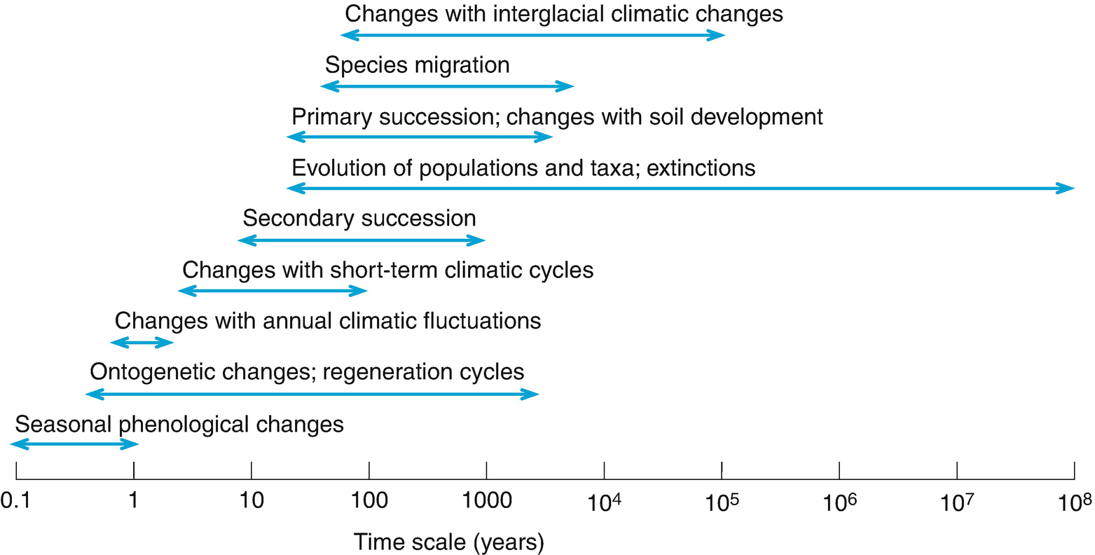
Time scales for dynamic changes in vegetation. (after Miles 1987)
17.3.1 Short-Term and Seasonal Vegetation Dynamics
Plants need to adapt to changing daily and seasonal conditions in their habitat, particularly periodic changes of radiation, day length and temperatures, as well as the amount and distribution of precipitation. The short-term dynamics of plants and vegetation units are considered by the discipline of phenology, the science of seasonal sequences of life cycles of plants and plant communities. Visible changes in the life cycles of plants are recorded, stages of development defined and attempts made to explain these by changes over time, as well as biotic and abiotic factors in the habitat. Of interest are not just typical sequences but also differences in weather conditions from year to year, which may have a considerable effect on the timing of flowering, conditions for germination, the amount and allocation of biomass production and formation of fruit and seeds, as well as the start and duration of individual phenological stages.
Box 17.2: Methods in Phenology Research
Phenological studies focus on the appearance of plants during their temporal development throughout the year. The characteristics include floral development (reproduction) and leaves (vegetative growth). In spring, observations are usually made weekly and later at longer intervals. The numbers of flowers, shoots, leaves and fruits, as well as the degree of cover, are typically counted or measured.
Dierschke (1994) provides an example of such analysis for deciduous trees in nemoral forests and reproductive stages in phenology.
Vegetative phenological stages
0. Buds completely closed
1. Buds with green tips
2. Green leaf emergence
3. Leaves 25% unfolded
4. Leaves 50% unfolded
5. Leaves 75% unfolded
6. Leaves fully expanded
7. First leaves yellowing
8. Leaves 50% turned colour
9. Leaves 75% turned colour
10. Leaves 75% turned colour
11. Bare
Reproductive phenological stages
0. Without flower buds
1. Flower buds recognisable
2. Flower buds swollen
3. Shortly before flowering
4. Start of flowering
5. Up to 25% flowers mature
6. Up to 50% flowers mature
7. Full flowering
8. Flowering decreasing
9. Flowering ceased
10. Fruiting
11. Fruit abscission
Comparable categories have been developed for herbs, grasses and cryptogams. For general phenological examination, in which the whole plant community is considered, permanent areas are marked and regularly monitored. This may include all or only selected species in vegetative and reproductive stages of development (phenophases). In addition, environmental data are recorded, particularly those related to weather conditions (temperature, precipitation). For the visualisation of these data sets, species are sorted by the start of flowering or the length of the flowering period.
Development during the year is often subdivided into phenophases that are based on phenological plant types. They have the same developmental rhythm, which appears in comparable leaf characteristics, time of flowering and duration of the vegetative period. The applicability of these types is limited to particular regions because individual species may behave differently in different communities. Phenophases are initiated by the start of flowering, leaf unfolding, leaf colouration and leaf abscission of particular plant species.

Phenological phases in growing season. Examples of an oat grass-Arrhenatherum-grassland in Poland, for trees and herbs in a mixed oak forest in northern Germany (with comparison of Ranunculus ficaria to those in Russia and England) and for plant species from cold regions (high mountains, arctic regions) and from semi-arid and arid regions (steppe, deserts). 1 Time required for complete leaf cover; 2 death due to drought; 3 flower buds visible; 4 flowering period; 5 fruit ripening and seed dispersal. (after Larcher 2003)
Phenological characteristics have been known for a long time and are relatively easy to observe. In the daily rhythm, leaves and petals move (heliotropism) in order, for example, to protect against excessive radiation or to capture the highest possible amount of radiation. The production of odorous substances, the secretion of nectar or the supply of pollen by flowers may be coupled with the active phases of animal partners and change during the day. This is mainly regulated by the daily photoperiod.

Flowering period of geophytes during spring in a hornbeam (Carpinus betulus) forest. (after Schmidt 1969)

Zonation of plant communities on borders of large wadis in North Yemen (Yemen Arab Republic), determined by different height of water flow. a Wadi Mawr in Tihama Mountains with highly variable water discharge during year (Photo: K. Müller-Hohenstein). b Schematic transect from bed of wadi to lower terraces and to top of wadi bank. Only therophytes such as Bacopa monnieri and Phyla nodiflora are able to colonise the frequently moving gravel banks. In the more strongly consolidated parts of the banks, grasses with particular root systems (rhizomes), such as Desmostachya bipinnata, and very elastic woody species, such as Tamarix nilotica, are able to survive episodic flooding. The resulting changes in vegetation are relatively rapid and aperiodic. (Deil and Müller-Hohenstein 1985)
Phases of activity and dormancy are characteristic of all regions with a seasonal climate. A distinction is made between phases of stronger activity of vegetative and reproductive growth. Occasionally, several vegetative pulses of growth occur, which can be detected as growth rings even in annual species (Schweingruber and Poschlod 2005). In late summer, some tree species rapidly form very distinct new shoots. Seasons may be determined by temperature or from the water supply. In the latter case, seasonal changes in water supply can prove to be the most important regulatory factor for the short-term dynamics of vegetation. In woody species, two types have evolved: Late flowering plants flower only after the development of leaves or after shedding of leaves at the end of the rainy season, while early flowering plants start to flower before the emergence of leaves, i.e. before the rainy season begins. Both types are adapted to the simultaneous occurrence of pollinators or seasonal periods with regular winds.
Because of the usually favourable conditions of temperature and moisture in the perhumid tropics, plants often grow continuously. Nevertheless, irregular bursts of growth may be observed, even with differences among different parts of individual plants. However, definite flowering periods or other phenological phases can hardly be established. Some individuals flower and carry ripe fruits at the same time. It is remarkable that several plant species only flower episodically, sometimes only after several decades.
The timing and duration of specific phenological phases within a year is very closely correlated with the sequence of weather conditions during the year. These short-term dynamics, occurring year by year, but not necessarily cyclical, are fluctuations. Changes are registered at the level of individual plants. The most important expression of fluctuation is a change in the dominance between co-occurring species. In contrast to successional dynamics, a return to the previous state is possible. In field studies, it is not easy to distinguish between fluctuation and succession because both overlap and influence each other. The phenological spectrum for species of woodland edges for two different annual sequences records the extent of such fluctuations (Fig. 17.24).

“Flowering desert” (Arabic, acheb) after one of the rare rainfall events in extreme deserts. Such an unpredictable change in vegetation is called a fluctuation; the plant community is composed of only therophytes. This example is from the Arabian Desert (United Arab Emirates) and contains Silene villosa, Senecio glaucus and Plantago amplexicaulis. (Photo: K. Müller-Hohenstein)

Phenological spectra for species on woodland edges. The small trapezoidal areas show the flowering period. (after Dierschke 1994)
Evaluations of synecological and biocoenological links are only emerging, for example, of the temporal niches of flowering species in plant communities, of the synchronisation of insects and animals that distribute pollen, fruits and seeds. This would not only make pollen calendars available for those with allergies but would also help protect nature, i.e. by providing dates for mowing, for extensive maintenance or as a control for the success of different types of land use.
17.3.2 Long-Term Vegetation Dynamics
Medium- and long-term changes in plant cover over several decades and up to millennia are analysed in research on successions. Only some decades ago, the principles and models of these successions were derived from empirical data. However, from the beginning there was controversy in the scientific discussions between those with a holistic approach who consider the complete ecosystem and those with a reductionist approach who focus on individual functions and processes in succession. Both approaches had the same aim in trying to recognise the causes of vegetation dynamics by explaining the resulting effects and predicting them. There remains a belief that there are basic rules of dynamic sequences, but many processes are now seen as stochastic. This is demonstrated by the influence of extreme climatic events such as prolonged drought (Kreyling et al. 2011). The necessity of considering spatial and temporal scales in greater detail is generally accepted.
Box 17.3: Methods for Studying Succession
Research on succession has followed two complementary paths. In one, the development of the vegetation over time is studied at a particular site, including experimental treatments. In the other approach, the focus is on the current spatial composition of vegetation, which is used to reconstruct changes over time (false time series, or space-for-time substitution). An example of this is the littoral zone of a lake, which in its spatial development may be seen as an ecological series, while its temporal processes at the same site may be interpreted as succession.
Indicator plants, the age structure and diversity of stands or an analysis of seed banks can often help to establish the temporal sequence of particular developmental stages. In addition, external indicators are often used, such as differences in soil profiles or historical records from archives or land-use registries and account books of farms, which often have data about fertilisation or the use of herbicides at particular times.
Nevertheless, there are inherent problems in drawing conclusions from space for time substitutions. Therefore, more direct methods of understanding successions are increasingly being used. Spatially limited units of vegetation are established and plant individuals are monitored in regular sequences (biomonitoring). This long-term observation on permanent plots provides detailed analysis about population dynamics as the vegetation changes. Evaluation of aerial photographs and repeated satellite data are increasingly being used, although the scale is often not sufficient for the observation of individuals. Quickbird, with a resolution down to 0.6 m (but only panchromatic), has some of the best satellite imaging capabilities. It can be used to make comparisons of the average performance of stands; the structural aspects of plant cover are most obvious, while inventories of species are often not comparable. Experimental studies of succession are carried out on comparable areas using a range of treatments (e.g. different fertiliser applications, mowing regimes, single or multiple soil tillage, fencing and exclusion of grazing or other sorts of herbivory), and the effects on the vegetation during the following period are measured. Biomonitoring is also used in applied analyses of succession for the regulation and modification of measures in nature conservation in order to depict future trends in the development of the vegetation.
17.3.2.1 Beginnings of Succession Research
Systematic research on vegetation dynamics is connected with the names of the ecologists Clements and Gleason. Clements (1916) is regarded as the founder of the discipline of successional research, starting from the idea that only undemanding species grow first on bare substrates. Once established, species change and influence the conditions and community of their site, which then facilitates invasion by others. Clear temporal periods are recognisable until the development of a uniform, final community, the so-called climax community, representing a relative equilibrium. Small fluctuations in community assemblages are possible, but a reversal of the clearly directed processes leading to this climax community is not.
Later Clements assumed three succession sequences. One of these sequences has its origin in a freshwater basin. During the processes of receding water and emerging land in temperate latitudes, deciduous forests develop as a climax via a boggy and pre-forest stage (hydroseries). Another sequence starts from a saline substrate (haloseries) and a third on bare rock (xeroseries), but all end in the same forest climax. Changes in the site always originate from plants themselves. Also, in larger areas with the same climatic conditions, the same final community will always emerge (monoclimax). This concept was well received, but there were critics who could not empirically confirm this theory. The reason for the discrepancy was that Clements concentrated on the dynamics of undisturbed vegetation (primary succession) and interferences of any kind, and developments arising from them (secondary succession), were disregarded.
Clements’ theory, which regarded plant communities as “organisms”, was rejected by Gleason (1926), who stressed that there was also an individualistic type of vegetation dynamics without clear steps and without formation of the different vegetation units. He started from the assumption that changes in species at a site depended on the species composition and the influx of diaspores to that site.
-
A relatively general interpretation of the broad spectrum of dynamic events in ecosystems
-
A recognition of the enormous complexity of conditions and attempts to clarify individual aspects
Definitions of succession or vegetation dynamics are today broader and more general. These dynamics comprise changes in structure and species in vegetation units in space and time. Short-term, daily and seasonal changes are included. All forms may be described by the term patch dynamics (Pickett and White 1985). Another general definition underlines the notion that successions are medium- to long-term dynamic processes in a directed, temporal sequence of plant communities in an ecosystem. It is often stressed that these sequences are irreversible—within limits—and predictable and may be triggered by endogenous or exogenous processes. During succession, self-organisation in the ecosystem (on the precondition that there is no disturbance) increases and a balance between primary production and mineralisation develops.
Odum (1980) lists a total of 24 different ecosystem characteristics that are able to change during a succession sequence. He regarded development as a well-ordered process resulting from changes caused by vegetation and ultimately leading to a stable ecosystem, where maximum functional interconnections are achieved. The hypothetical final state is understood as a complex community of organisms with complex links and interactions, in which once equilibrium is achieved, it can change again, for example, after a new disturbance.
However, successions are often also understood as stochastic processes, basically because the seed input in a biocoenosis at a site is random; the same applies to the germination and establishment rates or the availability of necessary safe sites and the occurrence of disturbance—their type, intensity and degree—which are generally not predictable.
17.3.2.2 Succession Types
Succession may be considered over large or small areas, with fast or slow changes. It may be directed or cyclical and may be affected by endogenous or exogenous processes, which may differ by type, intensity, duration or extent. It is important to consider the geographical location within different climatic zones and whether development occurs on newly formed soils or on those previously colonised. Finally, participating plant species will differ in their ability to disperse and compete and in their life history strategies and resource demands/strategies. Dynamic processes are triggered if net production and mineralisation in an ecosystem are not balanced. In such cases it is possible, for example, to accumulate organic matter (formation of bogs, autotrophic succession) or for organic matter to be consumed (use of humus by agricultural systems, heterotrophic succession).

Types of directed and cyclical vegetation dynamics. (after Jochimsen 1993)
Relationships between spatial and temporal dimensions in changes in vegetation
|
Individual |
Patch |
Population |
Community |
Landscape |
Region |
|
|---|---|---|---|---|---|---|
|
Fluctuation |
× |
×× |
×× |
|||
|
Gap dynamics |
× |
×× |
×× |
|||
|
Patch dynamics |
× |
× |
× |
|||
|
Cyclical succession |
× |
×× |
× |
|||
|
Regeneration succession |
×× |
×× |
×× |
|||
|
Secondary succession |
× |
×× |
×× |
×× |
||
|
Primary succession |
×× |
×× |
×× |
|||
|
Secular succession |
× |
× |
× |
Primary Successions

Different stages of primary succession. a On fresh volcanic lava dense moss and lichen communities have developed after 8 years. b Only specialists among the vascular plants (e.g. Pozoa volcanica) become established quickly on almost unweathered rocks without soil. c Only after several decades do the first trees (Nothofagus obliqua, N. dombeyi) form open woodland vegetation. Photos were taken on sites on Llaima Volcano in southern Chile. (Photos: K. Müller-Hohenstein)

Succession on moraines of Aletsch Glacier (Switzerland) (after Klötzli 1993)
Very few plants are able to cope with the hostile conditions of a site during the initial phases. On rocks, cryptogamic communities develop first, perhaps lithophilic lichens, then fruticose lichens, mosses and ferns. In unfavourable exposed positions, for example on steep rock walls or on mobile debris, development rarely goes beyond this phase (permanent pioneer communities). Usually, the pioneer communities, which themselves depend on the input of propagules from the surrounding areas, change the site over the course of time, which allows for the formation of a soil substrate. Many Leguminosae are herbaceous pioneers that facilitate the accumulation of nitrogen in this new substrate. Upon the establishment of later pioneer plants, these will help change the local microclimate. If flowering plants have not become established during the first phase of succession, they will now follow. These are predominantly heliophilic, epigaeically germinating annuals or, where climatic conditions do not allow such establishment, undemanding (i.e. able to grow on a nutrient-deficient substrate) herbaceous hemicryptophytes and chamaephytes.
As succession progresses, the pioneer species are excluded more and more with each step by more demanding species. When this change takes place solely because of the changes in the vegetation itself, it is called autogenic succession. If other causes are more important— for example, natural climate change or a lower groundwater table caused by human extraction of water—this is called allogenic succession. If successions proceed under steady external conditions, there are further stages, after the pioneer stage where competing species occur, that are superior to the pioneer species in vegetative and reproductive growth. These species grow taller, despite lower rates of growth, because of their longer life span (occurrence and increase of shrubs and trees), and they are more shade tolerant but often have less effective mechanisms for distribution, despite their more effective occupation of space in the long-term. Trees are superior to shrubs, forming polycormones, which enable them to dominate for a certain time. In the final phase of such development, trees dominate. This type of primary succession is understood to be progressive because the diversity increases at the level of the species as well as with regard to structure.

Main characteristics of progress of primary succession. Exemplified for silicate rock and under sub-Atlantic climatic conditions. T: Therophytes; H: Hemicryptophytes; G: Geophytes; C: Chamaephytes; P: Phanerophytes. (after Dierschke 1994)
Environmental changes during succession (after Klötzli 1993)
|
1. Species structure |
|
|
Species composition Number of autotrophic species (autotrophic diversity) Number of heterotrophic species (heterotrophic diversity) Species diversity Niche specialists Size of organism Life cycle Selection pressure Type of production |
First rapid, then stepwise change Increasing, often early in secondary succession Increasing, until late in secondary succession Initially increasing, then stable or again decreasing Initially broad then narrow Initially small then large Initially brief and simple, then long and complex Initially r-selection then K-selective Initially quantitative then qualitative |
|
2. Nutrient cycles |
|
|
Cycles Nutrient exchange Role of organic debris (detritus) |
Initially open then closed Initially rapid then slow Initially unimportant then very important |
|
3. Organic structure |
|
|
Total biomass Stratification Inorganic nutrients Recalcitrant organic material (e.g. humus) Biochemical diversity (e.g. pigments) Chlorophyll amount |
Initially small then large Initially one layer then multiple Initially in soil then in biomass Initially little then much Initially low then high (increasing accumulation of toxins!)Initially small then large (in secondary succession little difference!) |
|
4. Energy flow |
|
|
Relation to food chain Gross primary production Net primary productionTotal respiration Primary production per unit respiration Primary production per unit biomass Biomass per unit of energy |
Initially simple (food chain) then complex (food web) During early phase of primary succession increasing (only limited or no increase in secondary succession) Continuously decreasing Continuously increasing Initially primary production greater than equal to respiration (steady-state condition) Initially large then small Initially small then large; therefore, minimal use of energy per unit of biomass |
|
5. Homeostasis (ecological steady-state, result of irreversible processes) |
|
|
Internal symbiosis Nutrient storage Stability (resistance to disturbance) Entropy (increasing entropy) Information |
Initially not developed then developed Initially small then large Initially small then large Initially large (small) then small (constant) Initially small then large |
Disturbances and Secondary Successions
Primary successions occur faster under warm, humid climatic conditions than under cold or dry conditions. However, it is most important that development of these successions are not affected by disturbances, which can only be rarely excluded. Thus, primary successions are particularly important for a better understanding of the processes of secondary successions, which dominate the actual vegetation dynamics in our environment.

Secondary successions develop after disturbances, which may be natural, for example, a when dead wood accumulates after volcanic activity and subsequent fire in a forest community on the Lanin Volcano in southern Chile. However, b the disturbances can also be human-made, for example, forests cleared by fire for range lands, not for timber, in southern Chile near Aisen. (Photos: K. Müller-Hohenstein)
There are several definitions and a multitude of different types of disturbances (Box 17.4).
Box 17.4: Disturbances: Definitions and Properties
A disturbance is a relatively discrete event in time that concerns an ecosystem, community or population structure (of vegetation) and changes the resources, substrate availability or physical environment (Pickett and White 1985). Because this is an absolute definition, all changes must be measured and accounted for. In contrast, by some relative definitions, disturbances are regarded as events leading to deviations from the normal dynamics in an ecosystem or plant community, based on the assumption that a “normal” state is known. Furthermore, severe disturbances can range from having very far-reaching consequences, up to a complete floristically and structurally different plant community, to very small ones, for example, affecting the ability of a single plant to resprout.
Richter (1997) distinguishes between endogenous and exogenous disturbances. The former occur regularly; they are a feature of a system, so organisms in the community adapt. This is the case for seasonal changes and for changes such as frequent, regular flooding of meadows. Most disturbances that then lead to secondary successions are exogenous and are typically natural in origin (e.g. catastrophic storms or landslides and avalanches); however, they can also be caused by human activity.
To overcome the high complexity of disturbance regimes, Buhk et al. (2007) established a classification scheme that takes into account the disturbance type (e.g. felling, flooding), disturbance space, form and distribution (spatial dimensions) and disturbance frequency, seasonality and duration (time dimensions).
The intermediate disturbance hypothesis (IDH) puts forth an often discussed theoretical background to evaluate the effects of a given disturbance (Sect. 13.5 and Sect. 20.3). This hypothesis describes the relations between the type and force of the disturbance and the species diversity in the area concerned (Huston 1979). It states that at intermediate levels of disturbance, species diversity is at its highest. No species will be lost by being overly disturbed, and the competitive exclusion of a species is not very likely. Field tests of the IDH showed mixed support for and against this hypothesis (Mackey and Currie 2001).

Type and occurrence of disturbances in different ecozones. (after Böhmer and Richter 1996)
-
Disturbances may interrupt the dynamics and the vegetation but leave the ecosystem at a certain stage (permanent communities).
-
Changes occur without clear direction within vegetation, for example, because of long-term fluctuations in the water level.
Influences mentioned can lead to faster or slower, as well as irreversible, alterations. A response that reverses the process or sets it back to a previous step or direction of change is known as regressive succession. These include successions that occur as a consequence of over-exploitation or selective use of forests and pastures.
Most often secondary succession leads to reestablishment of the state that preeceded the disturbance. Here, too, the changes in direction lead to a more complex form of organisation in the plant community. However, secondary successions have different initial stages. Their dynamic changes start from an already settled substrate and may build on an existing seed bank. This means that secondary successions progress faster than primary successions; right from the start there is competition for space and resources, and only species that can compete are able to invade.

Successions on fallowed agricultural fields: influencing factors and interrelations. (after Schmidt 1993)
Secondary succession in fallow pastures is delayed because of the dense grass layer. Schreiber (1995) shows from observations over 20 years that the establishment of woody plants can occur in several ways. Occasionally, well-known basic processes in the succession of different functional types of plants from annuals to woody species occur. However, pastures, initially relatively homogeneous, often show the formation of dominance patterns with few species that cover the area well after just a few years. With good nutrient supply, herbs dominate because biomass is not removed (auto-eutrophication), but with poor nutrient supply grasses dominate. The temporal sequence of individual stages differs considerably. In some areas, 10–15 m high pre-forest vegetation occurs, while on other potential forest sites neither trees nor shrubs grow. The difference in the establishment of woody plants does not fit any succession model so far described; a prediction about changes in life forms and species is not yet possible, even if occasionally such phases in vegetation dynamics may be clearly seen.

Polycormophyte succession of woody species in grassland. 1 With establishment of low-growing woody species; 2 followed by tall-growing woody species; 3 with woody, tall trees. (after Dierschke 1994)
The concept of succession as a directed, more or less deterministic, although predictable, process must therefore be corrected according to empirical results obtained in recent decades. These changes over time are very complex, with many variables influencing development, for example, site, biological reproduction, space and time. Particularly important are the type, intensity and duration of disturbance. All these factors make it difficult to regulate and predict successions.
Cyclical Vegetation Dynamics

Succession in Mediterranean oak forest. a Cycles following clear felling. b Regression after multiple fires. (after Dierschke 1994)
-
A rejuvenating and juvenile phase, with young plants of the same or different tree species, with the previous phases occurring again. Often light-demanding trees invade first, followed by shade-tolerant trees.
-
An optimal phase corresponding to a forest of uniform age with few species, a closed stand with little undergrowth.
-
Ageing and decaying phases when the tree layer is disrupted over large areas and species requiring light are able to invade.
These phases may be regarded as a continuous process of self-thinning.

Mosaic cycle in tropical rainforest. Open tree crown pioneer species; thick tree crown canopy species; medium tree crown shade-tolerant species. (after Richter 1997)
Disturbance is again seen as the driving force for cyclic vegetation dynamics. The life span of “key organisms” is important, and competition following their death is centred on obtaining light and nutrients. The same is true for mechanical influences (wind breakage, fire). Constant conditions are not to be expected in a pristine forest, which is also a mosaic of asynchronous phases of cyclical vegetation dynamics. During the individual phases, the structural characteristics of forests and their species diversity change.
Today, additional types of cyclical vegetation dynamics are distinguished based on questions of scale and preferential occurrence in different biomes. The formation of mosaics over large areas in Hawaii is known as a consequence of the “death of cohorts” (Müller-Dombois 1995). Demographically unfavourable situations caused and maintained by fire and storm damage are the driving force. In this context, the mass die-off of bamboo-like grasses in all tropical regions should also be included. However, it is still not clear whether only endogenous (age) or also exogenous (climate) influences are responsible; it is likely that a combination of both is responsible.

Developmental phases of different types of plants during changes in vegetation. (after Richter 1997)
17.3.2.3 Aspects of Applied Succession Research

Pioneer plant species are able to start the succession in areas requiring protection, such as those subject to erosion. Pennisetum setaceum a is a tussock grass with extensive roots that is suitable for the stabilisation of steep slopes (mountains in Yemen Arab Republic). b As part of a project to protect against severe degradation of vegetation and soils in the Central Atlas Mountains (Morocco), a mixture of suitable plant species, such as dwarf and brushwood scrubs, dwarf palms and Opuntia cactus was used to achieve the initial stages in regeneration of area. (Photos: K. Müller-Hohenstein)
Today, we know about asynchronous vegetation cycles and therefore understand the limits to the practical application of current knowledge of vegetation dynamics. Management recommendations for the maintenance of certain ecosystems also need to be revisited, as do the minimum spatial dimensions of protected areas. Current knowledge of vegetation dynamics helps in the selection of “replacement areas”, where disturbed or lost communities may develop again.
Biomonitoring was developed in order to understand syndynamic processes, to identify damaging influences so that they could be quickly counteracted or minimised. Examples are the indication of air pollution and the eutrophication of water. Vegetation changes resulting from interventions at certain sites can also be recorded by continuous biomonitoring. Multiple scales on the hemeroby (level of naturalness) of spaces for vegetation have been devised. Red List species, loss of species, proportion of annuals and neophytes are important values for structuring vegetation units according to the degree of human intervention. Ultimately, knowledge about vegetation dynamics is applied in attempts to improve areas to be used for agriculture or forestry and to control such attempts. Thus, for example, the application of Ca-containing fertilisers in order to combat the acidification of soils in forests and the effects of herbicide application in vineyards, leading to the loss of endangered species, were assessed in this way.
17.3.3 Vegetation Dynamics and Strategy Models
Variability within a single plant can be considerable, growth can be fast or slow, tolerance to shade can be high or low, and dispersal from the parent plant can be far or near, to name a few parameters. Such characteristics, acquired during the course of evolution, enable plants to successfully compete with other individuals and to become established and are often summarised by the term “strategy”. It is defined as the sum of genetically fixed physiological and morphological adaptations required to cope with different environmental conditions, conquer a habitat and persist with optimal use of resources. Individual plants, populations and species are also classified using strategic aspects as plant functional types (Sect. 20.2).

Possible behaviour of two species over the course of succession. (after McCook 1994)
17.3.3.1 Initial Floristic Composition

Scheme of initial floristic composition model of succession. The curves show the behaviour of six different species. (after Finegan 1984)
17.3.3.2 r and K Strategies
The concept of r and K selection is based on models of population growth in animals, which was developed by MacArthur and Wilson (1967). This concept is used by botanists and zoologists to stress particularly contrasting characteristics of species. “r” is the intrinsic rate of population growth or rate of reproduction, while “K” represents the carrying capacity or maximum population size. Essentially, the r and K concepts stress the allocation patterns of limiting resources that are inversely related.
r-strategists form a large number of very small seeds representing a high proportion of their phytomass; they also tend to have an efficient mechanism for dispersal and grow fast without high biomass accumulation. This leads to a much quicker time to reach reproductive maturity, and such plants also tolerate long periods of seed dormancy, but the seeds can be activated very quickly. Species that are r-strategists are short-lived opportunists that are able to become established faster in their environment than shade-tolerant species, but they are inferior competitors to K-strategists.
K-strategists are long-lived and slow-growing and accumulate large amounts of biomass over time. For this reason, and because they are shade tolerant, they are able to outcompete r-strategists. They invest less into reproduction and will typically produce a small number of seeds that are larger than those of r-strategists. However, they need to form metabolites for defence to protect long-lived leaves and other organs from herbivory. In terms of successional stages, it is easy to determine that early stages are dominated by r-strategists, while later stages are dominated by K-strategists. On fallow land, for example, annual and biennial species are replaced over time by shrubs, which are then taken over by trees.

17.3.3.3 Strategy Types of Grime (C-S-R Model)
Grime (1974) and Grime et al. (1988) worked out one of the most well-known models of vegetation dynamics: the triangle model of primary ecological strategies. Stress tolerance, adaptation to unfavourable conditions and reaction to disturbance missing in the r/K strategy model were regarded as particularly important. Three strategy types were introduced (Sect. 19.3):
Competitor strategist (C): long-lived, competitive species on favourable sites without limitation of resources and almost stress free. They use resources particularly well, often possess storage organs and show considerable plasticity in root and shoot formation, continuously produce leaves that live for only a short time, and have low seed production. These are perennial herbs, shrubs and trees, which form in mid to late successional stages.
Stress-Tolerant Strategist (S): species adapted to unfavourable sites with limited or poor availability of resources (e.g. inadequate light, drought, nutrient deficiency, frequent frosts). They are long-lived, but with low productivity and reproductive rates and are often restricted to sites with little or no competition. Extremely stress-tolerant species are lichens on cold and dry sites.
Ruderal Strategist (R): short-lived, usually herbaceous species with fast growth rates and high seed production, usually self-pollinated with rapid seed ripening and dispersal, disturbance-tolerant opportunists and pioneers, but weak competitors. Therefore, they grow on sites with frequent, natural disturbances.
However, it is difficult to classify many plant species into only one of these three strategies. Intermediates are frequently observed, where plants with characteristics of several strategic types in different combinations are possible. On favourable sites where competitor strategists should dominate, C-R transition forms are found if the favourable conditions are temporarily disturbed, for example, by mowing meadows. Stress-tolerant competitor strategists (C-S) are long-lived species; for example, many tree species of nemoral forests have adapted to non-optimum sites. Stress-tolerant ruderal strategists (S-R) grow on unfavourable sites that are often disturbed. Included is also an intermediate type (C-S-R) combining several strategies and may also occur in temporal sequence within the same species.

C-S-R diagram of different types of strategy according to Grime. C competitor species; S stress-tolerant species; R ruderal and intermediate types with relative importance of competition (BC), stress (BS) and disturbance (BR). (after Grime et al. 1988)
17.3.3.4 Resource Ratio Model of Tilman
All plant species are limited in their distribution by resources, which are often difficult to acquire but are required for survival. A species is deemed successful in competition for such a limiting resource if it is able to reduce the level of nutrients to the lowest level (called R*), resulting in competitive exclusion (Sect. 19.3). Tilman (1982) developed this model to describe the growth of algae, while for terrestrial systems the assumption is made that the most important limiting resource is within the soil (typically nitrogen) or is light. Any limitation in either of these resources will lead to increased stress within the plant. Often, these resources are inversely related, that is, a low nitrogen supply is typically associated with favourable light conditions, and low light levels (in the understorey) are commonly found at sites with favourable conditions for plant nutrition. Gradients between those two extremes lead to succession stages where plants replace each other according to their demands and their specific competitiveness. Each species grows fastest and reproduces best with the resources to which it is best adapted and where it can outcompete other species. Sufficient root biomass is very important for obtaining sufficient nutrients in the soil, but also sufficient above-ground biomass is essential for light capture by producing leaves. In primary succession, species able to cope with a poor nitrogen supply typically exclude species that require a great deal of nitrogen. As time passes, however, soil nutrition gradually improves thanks to mineralisation and nitrogen input into the system. Now, species able to cope with less light are more competitive. This hypothesis is the basis of the resource ratio model or the nutrient-light relation model.

Relationship between competition and colonisation capability. a Curve represents a hypothetical interspecific trade-off between competitive ability. Each point on this curve could represent a distinct plant species. The five points shown are for species A, B, C, D, and E. b Species A–E will have qualitative successional dynamics because of their colonisation–competition trade-offs. c Successional dynamics of dominant grass species of Cedar Creek Natural History Area (after Tilman 1988). d Observed interdependence of competitive ability and colonisation rates for five dominant grasses of Cedar Creek Natural History Area. R* for nitrogen is the observed level to which monocultures of each species reduced the concentration of dissolved ammonium and nitrate on fertile, low-nitrogen soils (Tilman and Wedin 1991a). Lower R* values correspond to a greater competitive ability (Tilman and Wedin 1991b). The colonisation rate is inversely related to the years each species required to colonise newly abandoned fields at Cedar Creek Natural History Area. (after Tilman 1994)
From these models, the consequences for biodiversity within areas may be derived. The more heterogeneous a space to be colonised is—particularly regarding its environmental conditions (e.g. nutrients, light, water) and natural and anthropogenic disturbances—the more species are able to coexist. It follows that with increasing heterogeneity not only does biodiversity increase but, in the habitat, resources should ideally be available at intermediate levels (Sect. 20.3).
17.3.3.5 Facilitation-Tolerance-Inhibition Models of Connell and Slatyer
Competition for resources may change by type and amount over time, especially when disturbance regimes are considered. Connell and Slatyer (1977) pointed out that the driving force behind vegetation dynamics and stress is the issue of scale, where certain dynamics only occur at certain scales. As such, three models, or succession pathways, are considered (Box 17.5):
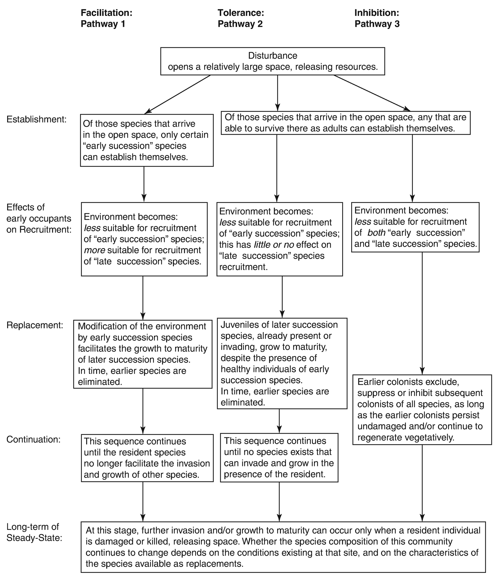
Facilitation model: Facilitation is understood as the “promotion” or “enabling” of other species, starting from the assumption that the first colonists change site conditions over the course of time autogenically in such a way (e.g. change in substrate, formation of humus) that colonisation by more demanding species is stimulated. This is usually linked to the displacement of the first colonists as they become unable to cope with the competitive advantage of the incoming species.
Tolerance model: Late successional species are neither stimulated nor inhibited. However, they are only able to establish themselves if previously established individuals die or are removed, leaving an area to invade. The species now present compete with one another and behave similarly to the resource ratio model of Tilman, where species with lower R* gain dominance.
Inhibition model: Earlier colonists suppress or inhibit subsequent invaders, which will only be able to become established in the event of a disturbance or by the creation of open space for short time spans due to an individual’s death and not because of their competitive advantage.
All three models have been tested in field experiments. The facilitation model may be observed in primary successions, where pioneer species prepare the substrate, as well as following disturbance, because the succession is thrown back into an earlier phase. Both of the other model versions were tested in later, species-rich successional stages. The final steady-state stage is regarded as relatively stable, but cyclical dynamics are not excluded.
Also, the question of stability is taken into consideration. Consequently, succession is regarded as a balancing reaction of a “stable” system that has been heavily disturbed. The spatial and temporal extent of the disturbance as well as their type and intensity are decisive for the following new initial stage of succession.
17.3.4 Vegetation Dynamics and Influence of Animals
At any time during succession, two important influences by animals must be taken into account (Sect. 19.4). The spectrum of species may be changed by herbivory, or at least the conditions for competition are changed. This is rarely fully taken into account because herbivores often eat seeds (granivores) and seedlings, and the extent of such disturbance is difficult to measure. Often it is a matter of speculation as to how vegetation would have developed without herbivory. However, animals are also vectors for propagules and, thus, for the distribution of species, and they participate decisively in the formation of spatial patterns and the composition of vegetation units. In addition, animals change site conditions by their excrement and by their mechanical activities and soil disturbance.
There is much evidence that animals, too, exhibit distinct dynamics. In the initial stages of succession, arthropod herbivores dominate, with 93% of all insect species; however, these proportions drop drastically within older successional stages (51%) and even more so in forest communities (44%). During the initial stages, sap-sucking phytophages make up half of that population, later only a quarter. Macro-invertebrates and predators associated with them increase with the age of the succession.

Adaptive strategies of plants and animals during secondary succession. (after Brown and Southwood 1987)
17.3.5 Further Aspects for Understanding Vegetation Dynamics
In addition to the concepts of vegetation dynamics mentioned so far, other ideas that incorporate the enormous complexity of ecosystems could be discussed, for example, those concerning convergence and divergence in the development of successions (Leps and Rejmanek 1991), the continuum concept by Austin (1985) or the discussion of chaos theory and non-linear systems (Stone and Ezrati 1996). These models, as well as those with partially overlapping concepts covered previously, show that it is not possible to describe all aspects of vegetation dynamics with “one simple formula”. Complex processes and patterns of vegetation dynamics may only be generalised or modelled to a certain extent. Descriptive models of the sequence of individual species are accepted, but they explain little. Also, little emphasis is placed on the fact that a species performs differently in juvenile stages than in older stages. As summarised by Bazzaz (1990: 258), “Despite much progress in modelling succession, the tension between simplicity of models for prediction and complexity to include all relevant parameters remains unsolved.”
A path towards a better understanding of processes and mechanisms of vegetation dynamics should integrate previous and new information from experimental approaches. Note should be made of different spatial and temporal scales, as well as of the organisational hierarchies of plants—individual, species, population, community. Recently, dynamic simulation models have been used to describe vegetation dynamics. In southern Ecuador, Dislich et al. (2009) used the FORMIND model to simulate the dynamics of tropical mountain forests and regarded this model as being well adapted to investigate disturbances to forest structure and species composition. The empirical results of long-term studies should be used for verification. For example, the results obtained by Schreiber (1995) on very detailed succession studies over more than 20 years (on fallow land) do not fit into any succession model. This means that succession can hardly be exactly predicted, and planning based on such predictions is risky.
17.4 Ecological Stability of Plant Communities and Disturbances
The topics of succession and cyclical vegetation dynamics touch on questions of the “stability” of plant communities and whole ecosystems, as well as the concept of ecological equilibrium, sometimes naively termed the “balance of nature”. Much controversy continues to surround this complex topic, particularly in relation to the definitions of stability and of the characteristics required for stability (Grimm et al. 1992). Temporal and spatial scales are often not considered sufficiently: stability is related to momentary conditions, years or centuries, of plant communities considering a span of only a few square centimetres up to many square kilometres. In all cases, stability/instability is linked to species interactions and demographic stochasticity (internal sources) or disturbance, environmental change and stress (external sources). The relations between stability and diversity or complexity are discussed in Sect 20.4.
Generally, definitions of ecological stability are linked to a system capable of maintaining its structures and functions over the long-term and that is properly used by humans. Population sizes of species may fluctuate little around a mean value, and turnover of species is possible to a limited extent (but not that of life forms or functional groups). Functional relations, such as within food webs, and the many different niches and feedback mechanisms in a system strongly determine stability. Theoretically, stability may thus be explained via the sum of all functional connections within a system. It is a dynamic concept that also includes the stability of processes. Stable systems react to disturbance and return to the initial stage by self-regulation. Ecological stability includes cyclical changes, but not successions. In contrast, a labile system is not able to withstand changing external influences.
-
Qualitative stability: property of a system that returns to its original state after a perturbation.
-
Resistance: a measure of the ability of a system to maintain its original state in the face of an external disturbance or perturbation.
-
Resilience: a measure of the speed at which a system returns to its original state after a perturbation.
-
Robustness: a measure of the amount of perturbation that a system can tolerate before switching to another state.
-
Variability: a phenomenological measure of the magnitude of temporal changes in a system property.
-
Persistence: a measure of the ability of a system to maintain itself through time.

Relations between different spatial scales (local, global) and stability. (after Begon et al. 1999)
-
Ecological stability, which includes the resistance of a system or its ability to return to its original state after a disturbance (resilience).
-
Ecological instability, where changes after a disturbance cannot be reversed.
-
Ecological lability, which is a transient phase with a strong disposition to change as a result of disturbance.

Basic types of ecological stability. These types differ according to the dynamics of chosen characteristics and to the presence or absence of external factors. (after Gigon 1982)

Basic types of ecological instability. These types differ according to the dynamic of chosen characteristics and to the presence or absence of external foreign factors. (after Gigon 1982)
Disturbances or perturbations are not necessarily negative for the stability of ecosystems or communities. They can even be essential for the maintenance of a dynamic ecological equilibrium. A boreal larch forest would develop into quite a different system without the regular influence of fires. The same interfering factors may thus have different consequences for a system. Disturbances may be seen as inherent properties of a system or as stochastic external events, the latter caused naturally or anthropogenically. Several years without precipitation in desert regions is an internal disturbance to the system, as is the regulation of population density based on predator–prey relationships, or the dynamics of avalanches in montane ecosystems. It is often difficult to distinguish between disturbances caused by endogenous biological processes and those caused by exogenous environmental influences. Variances in spatial and temporal scales must be taken into account. The scale extends from disturbances by continental drift, on a scale of millions of square kilometres taking millennia to occur, to damage by spring tides, late frosts or extreme herbivory affecting a few hectares over a much shorter time frame.
Finally, it must be stressed that there is no “balance of nature” in the sense of completely stable ecosystems: ecosystems are always dynamic and undergoing change. In addition, no value judgement is implied by the concept of ecological stability. A stable system might be judged differently by a farmer than by an environmentalist, by a skier differently than by a hunter. A practice-oriented synecology must include an evaluation of stability, which is based on accepted standards and models.
17.5 Summary
-
Beginning around the algae period / Eophyticum (about 4000 million years ago), the development of plants began with single-cell prokaryotes, which developed into algae. At the beginning of the Palaeozoic Period (about 450 million years ago), the first ferns and gymnosperms evolved. This development was largely influenced by geologic-tectonic and climatic events. It wasn’t until the Cretaceous Period (about 95 million years ago) when angiosperms completed the current flora arrangement, which remained quite uniform on the existing continents for a while. A diversification of the flora into plant kingdoms only developed in the Tertiary Period (30 million years ago).
-
A worldwide climatic cooling and periodic alternations between cold and warm periods in the Pleistocene (0.5 million years ago) were responsible for further vegetation change and discrete spatial separation of plant communities. Large disjunctions of species over hundreds of kilometres in latitude and in altitude are geographical vicariants resulting from these climatic fluctuations.
-
However, the present-day global and regional differentiation of the plant cover can only be understood by taking into account the direct and indirect, intended or unintentional influences of humans. Completely undisturbed plant communities no longer exist. Plant species are going and will continue to go extinct, and neophytes are spreading and dominating. In this chapter, examples from Central Europe, the Mediterranean, Saharan and tropical environments were presented in detail.
-
General models of short- and long-term vegetation dynamics have been elaborated. In short-term dynamics, the daily and seasonal processes are best known (phenology). Long-term dynamics include successions. Of general importance for successional dynamics are developments on bare soil and without any disturbance (primary succession). However, most successions are secondary following more or less regular natural or human-caused disturbances. There are several models for these dynamics (mosaic cycles, cohort dynamics and others). Different strategy models (r and K, CSR, resource-ratio and facilitation-tolerance-inhibition model) can also be related to successional dynamics. In this context the different facets of ecological stability are discussed, which include qualitative stability, resistance, resilience, robustness, variability and persistence.