Extragalactic Astronomy and Cosmology Peter Schneider

A: The electromagnetic radiation field

In this appendix, we will briefly review the most important properties of a radiation field. We thereby assume that the reader has encountered these quantities already in a different context.

A.1 Parameters of the radiation field

The electromagnetic radiation field is described by the specific intensity I _ν , which is defined as follows. Consider a surface element of area d A . The radiation energy which passes through this area per time interval d t from within a solid angle element d ω around a direction described by the unit vector ${\boldsymbol n}$ , with frequency in the range between ν and ν + d ν , is

$\displaystyle{ \mathrm{d}E = I_{\nu }\,\mathrm{d}A\,\cos \theta \,\mathrm{d}t\,\mathrm{d}\omega \,\mathrm{d}\nu \;, }$

(A.1)

where θ describes the angle between the direction ${\boldsymbol n}$ of the light and the normal vector of the surface element. Then, d A cos θ is the area projected in the direction of the infalling light. The specific intensity depends on the considered position (and, in time-dependent radiation fields, on time), the direction ${\boldsymbol n}$ , and the frequency ν . With the definition ( A.1 ), the dimension of I _ν is energy per unit area, time, solid angle, and frequency, and it is typically measured in units of $\mathrm{erg\,cm^{-2}\,s^{-1}\,ster^{-1}\,Hz^{-1}}$ . The specific intensity of a cosmic source describes its surface brightness.

The specific net flux F _ν passing through an area element is obtained by integrating the specific intensity over all solid angles,

$\displaystyle{ F_{\nu } =\int \mathrm{ d}\omega \;I_{\nu }\,\cos \theta \;. }$

(A.2)

The flux that we receive from a cosmic source is defined in exactly the same way, except that cosmic sources usually subtend a very small solid angle on the sky. In calculating the flux we receive from them, we may therefore drop the factor cos θ in ( A.2 ); in this context, the specific flux is also denoted as S _ν . However, in this Appendix (and only here!), the notation S _ν will be reserved for another quantity. The flux is measured in units of $\mathrm{erg\,cm^{-2}\,s^{-1}\,Hz^{-1}}$ . If the radiation field is isotropic, F _ν vanishes. In this case, the same amount of radiation passes through the surface element in both directions.

The mean specific intensity J _ν is defined as the average of I _ν over all angles,

$\displaystyle{ J_{\nu } = \frac{1} {4\pi }\int \mathrm{d}\omega \;I_{\nu }\;, }$

(A.3)

so that, for an isotropic radiation field, I _ν = J _ν . The specific energy density u _ν is related to J _ν according to

$\displaystyle{ u_{\nu } = \frac{4\pi } {c}J_{\nu }\;, }$

(A.4)

where u _ν is the energy of the radiation field per volume element and frequency interval, thus measured in $\mathrm{erg\,cm^{-3}\,Hz^{-1}}$ . The total energy density of the radiation is obtained by integrating u _ν over frequency. In the same way, the intensity of the radiation is obtained by integrating the specific intensity I _ν over ν .

A.2 Radiative transfer

The specific intensity of radiation in the direction of propagation between source and observer is constant, as long as no emission or absorption processes are occurring. If s measures the length along a line-of-sight, the above statement can be formulated as

$\displaystyle{ \frac{\mathrm{d}I_{\nu }} {\mathrm{d}s} = 0\;. }$

(A.5)

An immediate consequence of this equation is that the surface brightness of a source is independent of its distance. The observed flux of a source depends on its distance, because the solid angle, under which the source is observed, decreases with the square of the distance, F _ν ∝ D ⁻² [see ( A.2 )]. However, for light propagating through a medium, emission and absorption (or scattering of light) occurring along the path over which the light travels may change the specific intensity. These effects are described by the equation of radiative transfer

$\displaystyle{ \frac{\mathrm{d}I_{\nu }} {\mathrm{d}s} = -\kappa _{\nu }\,I_{\nu } + j_{\nu }\;. }$

(A.6)

The first term describes the absorption of radiation and states that the radiation absorbed within a length interval d s is proportional to the incident radiation. The factor of proportionality is the absorption coefficient κ _ν , which has the unit of cm ⁻¹ . The emission coefficient j _ν describes the energy that is added to the radiation field by emission processes, having a unit of $\mathrm{erg\,cm^{-3}\,s^{-1}\,Hz^{-1}\,\mathrm{ster}^{-1}}$ ; hence, it is the radiation energy emitted per volume element, time interval, frequency interval, and solid angle. Both, κ _ν and j _ν depend on the nature and state (such as temperature, chemical composition) of the medium through which light propagates.

The absorption and emission coefficients both account for true absorption and emission processes, as well as the scattering of radiation. Indeed, the scattering of a photon can be considered as an absorption that is immediately followed by an emission of a photon.

The optical depth τ _ν along a line-of-sight is defined as the integral over the absorption coefficient,

$\displaystyle{ \tau _{\nu }(s) =\int _{ s_{0}}^{s}\mathrm{d}s^{{\prime}}\;\kappa _{ \nu }(s^{{\prime}})\;, }$

(A.7)

where s ₀ denotes a reference point on the sightline from which the optical depth is measured. Dividing ( A.6 ) by κ _ν and using the relation d τ _ν = κ _ν d s in order to introduce the optical depth as a new variable along the light ray, the equation of radiative transfer can be written as

$\displaystyle{ \frac{\mathrm{d}I_{\nu }} {\mathrm{d}\tau _{\nu }} = -I_{\nu } + S_{\nu }\;, }$

(A.8)

where the source function

$\displaystyle{ S_{\nu } = \frac{j_{\nu }} {\kappa _{\nu }} }$

(A.9)

is defined as the ratio of the emission and absorption coefficients. In this form, the equation of radiative transport can be formally solved; as can easily be tested by substitution, the solution is

$\displaystyle\begin{array}{rcl} I_{\nu }(\tau _{\nu })& =& I_{\nu }(0)\,\exp \left (-\tau _{\nu }\right ) \\ & +& \int _{0}^{\tau _{\nu }}\mathrm{d}\tau _{\nu }^{{\prime}}\;\exp \left (\tau _{\nu }^{{\prime}}-\tau _{\nu }\right )\,S_{\nu }(\tau _{\nu }^{{\prime}})\;.{}\end{array}$

(A.10)

This equation has a simple interpretation. If I _ν (0) is the incident intensity, it will have decreased by absorption to a value $I_{\nu }(0)\,\exp \left (-\tau _{\nu }\right )$ after an optical depth of τ _ν . On the other hand, energy is added to the radiation field by emission, accounted for by the τ ^′ -integral. Only a fraction $\exp \left (\tau _{\nu }^{{\prime}}-\tau _{\nu }\right )$ of this additional energy emitted at τ ^′ reaches the point τ , the rest is absorbed.

In the context of ( A.10 ), we call this a formal solution for the equation of radiative transport. The reason for this is based on the fact that both the absorption and the emission coefficient depend on the physical state of the matter through which radiation propagates, and in many situations this state depends on the radiation field itself. For instance, κ _ν and j _ν depend on the temperature of the matter, which in turn depends, by heating and cooling processes, on the radiation field it is exposed to. Hence, one needs to solve a coupled system of equations in general: on the one hand the equation of radiative transport, and on the other hand the equation of state for matter. In many situations, very complex problems arise from this, but we will not consider them further in the context of this book.

A.3 Blackbody radiation

For matter in thermal equilibrium, the source function S _ν is solely a function of the matter temperature,

$\displaystyle{ S_{\nu } = B_{\nu }(T)\;,\;\mathrm{or}\;\;j_{\nu } = B_{\nu }(T)\,\kappa _{\nu }\;, }$

(A.11)

independent of the composition of the medium (Kirchhoff’s law). We will now consider radiation propagating through matter in thermal equilibrium at constant temperature T . Since in this case S _ν = B _ν ( T ) is constant, the solution ( A.10 ) can be written in the form

$\displaystyle\begin{array}{rcl} I_{\nu }(\tau _{\nu })& =& I_{\nu }(0)\,\exp \left (-\tau _{\nu }\right ) \\ & & +B_{\nu }(T)\int _{0}^{\tau _{\nu }}\mathrm{d}\tau _{\nu }^{{\prime}}\;\exp \left (\tau _{\nu }^{{\prime}}-\tau _{\nu }\right ) \\ & =& I_{\nu }(0)\,\exp \left (-\tau _{\nu }\right ) + B_{\nu }(T)\,\left [1 -\exp \left (-\tau _{\nu }\right )\right ]\;.{}\end{array}$

(A.12)

From this it follows that I _ν = B _ν ( T ) is valid for sufficiently large optical depth τ _ν . The radiation propagating through matter which is in thermal equilibrium is described by the function B _ν ( T ) if the optical depth is sufficiently large, independent of the composition of the matter. A specific case of this situation can be illustrated by imagining the radiation field inside a box whose opaque walls are kept at a constant temperature T . Due to the opaqueness of the walls, their optical depth is infinite, hence the radiation field within the box is given by I _ν = B _ν ( T ). This is also valid if the volume is filled with matter, as long as the latter is in thermal equilibrium at temperature T . For these reasons, this kind of radiation field is also called blackbody radiation.

The function B _ν ( T ) was first obtained in 1900 by Max Planck, and in his honor, it was named the Planck function ; it reads

$\displaystyle{ B_{\nu }(T) = \frac{2h_{\mathrm{P}}\nu ^{3}} {c^{2}} \frac{1} {\mathrm{e}^{h_{\mathrm{P}}\nu /k_{\mathrm{B}}T} - 1}\;, }$

(A.13)

where $h_{\mathrm{P}} = 6.625 \times 10^{-27}\,\mathrm{erg}\,\mathrm{s}$ is the Planck constant and $k_{\mathrm{B}} = 1.38 \times 10^{-16}\,\mathrm{erg}\,\mathrm{K}^{-1}$ is the Boltzmann constant. The shape of the spectrum (Fig. A.1 ) can be derived from statistical physics. Blackbody radiation is defined by I _ν = B _ν ( T ), and thermal radiation by S _ν = B _ν ( T ). For large optical depths in the case of thermal radiation, the specific intensity converges to blackbody radiation. For small optical depth, the radiation field is approximated by an integral over the emissivity j _ν , which can deviate strongly from that of blackbody spectrum even in the case of a thermal source; an example is the optically thin bremsstrahlung from the hot gas in galaxy clusters (see Sect. 6.4 ).

/epubstore/S/P-Schneider/Extragalactic-Astronomy-And-Cosmology/OEBPS/A129044_2_En_BookBackmatter_Fig1_HTML.jpg

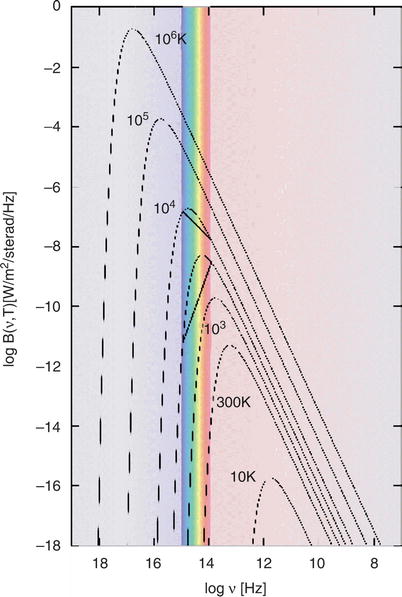
Fig. A.1

The Planck function ( A.13 ) for different temperatures T . The plot shows B _ν ( T ) as a function of frequency ν , where high frequencies are plotted towards the left (thus large wavelengths towards the right). The exponentially decreasing Wien part of the spectrum is visible on the left , the Rayleigh–Jeans part on the right . The shape of the spectrum in the Rayleigh–Jeans part is independent of the temperature, which is determining the amplitude however. Credit: T. Kaempf & M. Altmann, Argelander-Institut für Astronomie, Universität Bonn

The Planck function has its maximum at

$\displaystyle{ \frac{h_{\mathrm{P}}\nu _{\mathrm{max}}} {k_{\mathrm{B}}T} \approx 2.82\;, }$

(A.14)

i.e., the frequency of the maximum is proportional to the temperature. This property is called Wien’s law . This law can also be written in more convenient units,

$\displaystyle{ \nu _{\mathrm{max}} = 5.88 \times 10^{10}\,\mathrm{Hz}\; \frac{T} {1\,K}\;. }$

(A.15)

The Planck function can also be formulated depending on wavelength $\lambda = c/\nu$ , such that B _λ ( T ) d λ = B _ν ( T ) d ν ,

$\displaystyle{ B_{\lambda }(T) = \frac{2h_{\mathrm{P}}c^{2}/\lambda ^{5}} {\exp \left (h_{\mathrm{P}}c/\lambda k_{\mathrm{B}}T\right ) - 1}\;. }$

(A.16)

Two limiting cases of the Planck function are of particular interest. For low frequencies, h _P ν ≪ k _B T , one can apply the expansion of the exponential function for small arguments in ( A.13 ). The leading-order term in this expansion then yields

$\displaystyle{ B_{\nu }(T) \approx B_{\nu }^{\mathrm{RJ}}(T) = \frac{2\nu ^{2}} {c^{2}} \,k_{\mathrm{B}}T\;, }$

(A.17)

which is called the Rayleigh–Jeans approximation of the Planck function. We point out that the Rayleigh–Jeans equation does not contain the Planck constant, and this law had been known even before Planck derived his exact equation. In the other limiting case of very high frequencies, h _P ν ≫ k _B T , the exponential factor in the denominator in ( A.13 ) becomes very much larger than unity, so that we obtain

$\displaystyle{ B_{\nu }(T) \approx B_{\nu }^{\mathrm{W}}(T) = \frac{2h_{\mathrm{P}}\nu ^{3}} {c^{2}} \,\mathrm{e}^{-h_{\mathrm{P}}\nu /k_{\mathrm{B}}T}\;, }$

(A.18)

called the Wien approximation of the Planck function.

The energy density of blackbody radiation depends only on the temperature, of course, and is calculated by integration over the Planck function,

$\displaystyle{ u = \frac{4\pi } {c}\int _{0}^{\infty }\mathrm{d}\nu \;B_{\nu }(T) = \frac{4\pi } {c}\;B(T) = a\,T^{4}\;, }$

(A.19)

where we defined the frequency-integrated Planck function

$\displaystyle{ B(T) =\int _{ 0}^{\infty }\mathrm{d}\nu \;B_{\nu }(T) = \frac{a\,c} {4\pi } \,T^{4}\;, }$

(A.20)

and where the constant a has the value

$\displaystyle{ a = \frac{8\pi ^{5}k_{\mathrm{B}}^{4}} {15c^{3}h_{\mathrm{P}}^{3}} = 7.56 \times 10^{-15}\,\mathrm{erg\,cm^{-3}\,K^{-4}}\;. }$

(A.21)

The flux which is emitted by the surface of a blackbody per unit area is given by

$\displaystyle{ F =\int _{ 0}^{\infty }\mathrm{d}\nu \;F_{\nu } =\pi \int _{ 0}^{\infty }\mathrm{d}\nu \;B_{\nu }(T) =\pi B(T) =\sigma _{\mathrm{ SB}}T^{4}\;, }$

(A.22)

where the Stefan–Boltzmann constant σ _SB has a value of

$\displaystyle{ \sigma _{\mathrm{SB}} = \frac{ac} {4} = \frac{2\pi ^{5}k_{\mathrm{B}}^{4}} {15c^{2}h_{\mathrm{P}}^{3}} = 5.67 \times 10^{-5}\,\mathrm{erg\,cm^{-2}\,K^{-4}\,s^{-1}}\;. }$

(A.23)

A.4 The magnitude scale

Optical astronomy was being conducted well before methods of quantitative measurements became available. The brightness of stars had been cataloged more than 2000 years ago, and their observation goes back as far as the ancient world. Stars were classified into magnitudes, assigning a magnitude of 1 to the brightest stars and higher magnitudes to the fainter ones. Since the apparent magnitude as perceived by the human eye scales roughly logarithmically with the radiation flux (which is also the case for our hearing), the magnitude scale represents a logarithmic flux scale. To link these visually determined magnitudes in historical catalogs to a quantitative measure, the magnitude system has been retained in optical astronomy, although with a precise definition. Since no historical astronomical observations have been conducted in other wavelength ranges, because these are not accessible to the unaided eye, only optical astronomy has to bear the historical burden of the magnitude system.

A.4.1 Apparent magnitude

We start with a relative system of flux measurements by considering two sources with fluxes S ₁ and S ₂ . The apparent magnitudes of the two sources, m ₁ and m ₂ , then behave according to

$\displaystyle{ m_{1} - m_{2} = -2.5\,\log \left (\frac{S_{1}} {S_{2}}\right )\;;\quad \frac{S_{1}} {S_{2}} = 10^{-0.4(m_{1}-m_{2})}\;. }$

(A.24)

This means that the brighter source has a smaller apparent magnitude than the fainter one: the larger the apparent magnitude, the fainter the source. ¹ The factor of 2.5 in this definition is chosen so as to yield the best agreement of the magnitude system with the visually determined magnitudes. A difference of | Δ m | = 1 in this system corresponds to a flux ratio of ∼ 2. 51, and a flux ratio of a factor 10 or 100 corresponds to 2.5 or 5 magnitudes, respectively.

A.4.2 Filters and colors

Since optical observations are performed using a combination of a filter and a detector system, and since the flux ratios depend, in general, on the choice of the filter (because the spectral energy distribution of the sources may be different), apparent magnitudes are defined for each of these filters. The most common filters are shown in Fig. A.2 and listed in Table A.1 , together with their characteristic wavelengths and the widths of their transmission curves. The apparent magnitude for a filter X is defined as m _X , frequently written as X . Hence, for the B-band filter, m _B ≡ B .

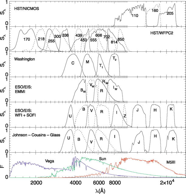
/epubstore/S/P-Schneider/Extragalactic-Astronomy-And-Cosmology/OEBPS/A129044_2_En_BookBackmatter_Fig2_HTML.jpg

Fig. A.2

Transmission curves of various filter-detector systems. From top to bottom : the filters of the NICMOS camera and the WFPC2 on-board HST, the Washington filter system, the filters of the EMMI instrument at ESO’s NTT, the filters of the WFI at the ESO/MPG 2.2-m telescope and those of the SOFI instrument at the NTT, and the Johnson-Cousins filters. In the bottom diagram, the spectra of three stars with different effective temperatures are displayed. Source: L. Girardi et al. 2002, Theoretical isochrones in several photometric systems. I. Johnson-Cousins-Glass, HST/WFPC2, HST/NICMOS, Washington, and ESO Imaging Survey filter sets , A&A 391, 195, p. 204, Fig. 3. ©ESO. Reproduced with permission

Next, we need to specify how the magnitudes measured in different filters are related to each other, in order to define the color indices of sources. For this purpose, a particular class of stars is used, main-sequence stars of spectral type A0, of which the star Vega is an archetype. For such a star, by definition, $U = B = V = R = I =\ldots$ , i.e., every color index for such a star is defined to be zero.

For a more precise definition, let T _X ( ν ) be the transmission curve of the filter-detector system. T _X ( ν ) specifies which fraction of the incoming photons with frequency ν are registered by the detector. The apparent magnitude of a source with spectral flux S _ν is then

$\displaystyle{ m_{X} = -2.5\log \left (\frac{\int \mathrm{d}\nu \;T_{X}(\nu )\,S_{\nu }} {\int \mathrm{d}\nu \;T_{X}(\nu )} \right ) +\mathrm{ const.}\;, }$

(A.25)

where the constant needs to be determined from reference stars.

Another commonly used definition of magnitudes is the AB system. In contrast to the Vega magnitudes, no stellar spectral energy distribution is used as a reference here, but instead one with a constant flux at all frequencies, $S_{\nu }^{\mathrm{ref}} = S_{\nu }^{\mathrm{AB}} = 2.89 \times 10^{-21}\,\mathrm{erg\,s^{-1}\,cm^{-2}\,Hz^{-1}}$ . This value has been chosen such that A0 stars like Vega have the same magnitude in the original Johnson-V-band as they have in the AB system, m _V ^AB = m _V . With ( A.25 ), one obtains for the conversion between the two systems

$\displaystyle\begin{array}{rcl} m_{\mathrm{AB}\rightarrow \mathrm{Vega}}&:=& m_{X}^{\mathrm{AB}} - m_{ X}^{\mathrm{Vega}} \\ & =& -2.5\,\log \left ( \frac{\int \mathrm{d}\nu \;T_{X}(\nu )\,S_{\nu }^{\mathrm{AB}}} {\int \mathrm{d}\nu \;T_{X}(\nu )\,S_{\nu }^{\mathrm{Vega}}}\right ){}\end{array}$

(A.26)

For the filters at the ESO Wide-Field Imager, which are designed to resemble the Johnson set of filters, the following prescriptions are then to be applied: $U_{\mathrm{AB}} = U_{\mathrm{Vega}} + 0.80$ ; $B_{\mathrm{AB}} = B_{\mathrm{Vega}} - 0.11$ ; V _AB = V _Vega ; $R_{\mathrm{AB}} = R_{\mathrm{Vega}} + 0.19$ ; $I_{\mathrm{AB}} = I_{\mathrm{Vega}} + 0.59$ .

Table A.1

For some of the best-established filter systems—Johnson, Strömgren, and the filters of the Sloan Digital Sky Surveys—the central (more precisely, the effective) wavelengths and the widths of the filters are listed

$\begin{array}{@{}lllllllllll@{}}\hline\mathbf{Johnson} & \mathrm{U} & \mathrm{B} & \mathrm{V} & \mathrm{R} & \mathrm{I} & \mathrm{J} & \mathrm{H} & \mathrm{K} & \mathrm{L} & \mathrm{M} \\ \hline\lambda _{\mathrm{eff}}\mathrm{(nm)} & 367 & 436 & 545 & 638 & 797 & 1220 & 1630 & 2190 & 3450 & 4750 \\ \varDelta \lambda \mathrm{(nm)} & 66 & 94 & 85 & 160 & 149 & 213 & 307 & 39 & 472 & 460 \\ \hline\end{array}$
$\begin{array}{@{}lllllll@{}}\hline\mathbf{Str}\ddot{\mathbf{o}}\mathbf{mgren} & \mathrm{u} & \mathrm{v} & \mathrm{b} & \mathrm{y} & \beta _{w} & \beta _{n} \\ \hline\lambda _{\mathrm{eff}}\mathrm{(nm)} & 349 & 411 & 467 & 547 & 489 & 489 \\ \varDelta \lambda \mathrm{(nm)} & 30 & 19 & 18 & 23 & 15 & 3 \\ \hline\end{array}$
$\begin{array}{@{}llllll@{}}\hline\mathbf{SDSS} & \mathrm{u}' & \mathrm{g}' & \mathrm{r}' & \mathrm{i}' & \mathrm{z}' \\ \hline\lambda _{\mathrm{eff}}\mathrm{(nm)} & 354 & 477 & 623 & 762 & 913 \\ \varDelta \lambda \mathrm{(nm)} & 57 & 139 & 138 & 152 & 95 \\ \hline\end{array}$

A.4.3 Absolute magnitude

The apparent magnitude of a source does not in itself tell us anything about its luminosity, since for the determination of the latter we also need to know its distance D in addition to the radiative flux. Let L _ν be the specific luminosity of a source, i.e., the energy emitted per unit time and per unit frequency interval, then the flux is given by (note that from here on we switch back to the notation where S denotes the flux, which was denoted by F earlier in this appendix)

$\displaystyle{ S_{\nu } = \frac{L_{\nu }} {4\pi D^{2}}\;, }$

(A.27)

where we implicitly assumed that the source emits isotropically. Having the apparent magnitude as a measure of S _ν (at the frequency ν defined by the filter which is applied), it is desirable to have a similar measure for L _ν , specifying the physical properties of the source itself. For this purpose, the absolute magnitude is introduced, denoted as M _X , where X refers to the filter under consideration. By definition, M _X is equal to the apparent magnitude of a source if it were to be located at a distance of 10 pc from us. The absolute magnitude of a source is thus independent of its distance, in contrast to the apparent magnitude. With ( A.27 ) we find for the relation of apparent to absolute magnitude

$\displaystyle{ m_{X} - M_{X} = 5\log \left ( \frac{D} {1\,\mathrm{pc}}\right ) - 5 \equiv \mu \;, }$

(A.28)

where we have defined the distance modulus μ in the final step. Hence, the latter is a logarithmic measure of the distance of a source: μ = 0 for D = 10 pc, μ = 10 for D = 1 kpc, and μ = 25 for D = 1 Mpc. The difference between apparent and absolute magnitude is independent of the filter choice, and it equals the distance modulus if no extinction is present. In general, this difference is modified by the wavelength- (and thus filter-)dependent extinction coefficient—see Sect. 2.2.4 .

A.4.4 Bolometric parameters

The total luminosity L of a source is the integral of the specific luminosity L _ν over all frequencies. Accordingly, the total flux S of a source is the frequency-integrated specific flux S _ν . The apparent bolometric magnitude m _bol is defined as a logarithmic measure of the total flux,

$\displaystyle{ m_{\mathrm{bol}} = -2.5\log S +\mathrm{ const.}\;, }$

(A.29)

where here the constant is also determined from reference stars. Accordingly, the absolute bolometric magnitude is defined by means of the distance modulus, as in ( A.28 ). The absolute bolometric magnitude depends on the bolometric luminosity L of a source via

$\displaystyle{ M_{\mathrm{bol}} = -2.5\log L +\mathrm{ const.}\;. }$

(A.30)

The constant can be fixed, e.g., by using the parameters of the Sun: its apparent bolometric magnitude is $m_{\odot \mathrm{bol}} = -26.83$ , and the distance of one Astronomical Unit corresponds to a distance modulus of $\mu = -31.47$ . With these values, the absolute bolometric magnitude of the Sun becomes

$\displaystyle{ M_{\odot \mathrm{bol}} = m_{\odot \mathrm{bol}}-\mu = 4.74\;, }$

(A.31)

so that ( A.30 ) can be written as

$\displaystyle{ M_{\mathrm{bol}} = 4.74 - 2.5\log \left ( \frac{L} {L_{\odot }}\right )\;, }$

(A.32)

and the luminosity of the Sun is then

$\displaystyle{ L_{\odot } = 3.85 \times 10^{33}\,\mathrm{erg\,s^{-1}}\;. }$

(A.33)

The direct relation between bolometric magnitude and luminosity of a source can hardly be exploited in practice, because the apparent bolometric magnitude (or the flux S ) of a source cannot be observed in most cases. For observations of a source from the ground, only a limited window of frequencies is accessible. Nevertheless, in these cases one also likes to quantify the total luminosity of a source. For sources for which the spectrum is assumed to be known, like for many stars, the flux from observations at optical wavelengths can be extrapolated to larger and smaller wavelengths, and so m _bol can be estimated. For galaxies or AGNs, which have a much broader spectral distribution and which show much more variation between the different objects, this is not feasible. In these cases, the flux of a source in a particular frequency range is compared to the flux the Sun would have at the same distance and in the same spectral range. If M _X is the absolute magnitude of a source measured in the filter X, the X-band luminosity of this source is defined as

$\displaystyle{ L_{X} = 10^{-0.4(M_{X}-M_{\odot X})}\,L_{ \odot X}\;. }$

(A.34)

Thus, when speaking of, say, the ‘blue luminosity of a galaxy’, this is to be understood as defined in ( A.34 ). For reference, the absolute magnitude of the Sun in optical filters is M _⊙U = 5. 55, M _⊙B = 5. 45, M _⊙V = 4. 78, M _⊙R = 4. 41, and M _⊙I = 4. 07.

B: Properties of stars

In this appendix, we will summarize the most important properties of stars as they are required for understanding the contents of this book. Of course, this brief overview cannot replace the study of other textbooks in which the physics of stars is covered in much more detail.

B.1 The parameters of stars

To a good approximation, stars are gas spheres, in the cores of which light atomic nuclei are transformed into heavier ones (mainly hydrogen into helium) by thermonuclear processes, thereby producing energy. The external appearance of a star is predominantly characterized by its radius R and its characteristic temperature T . The properties and evolution of a star depend mainly on its mass M .

In a first approximation, the spectral energy distribution of the emission from a star can be described by a blackbody spectrum. This means that the specific intensity I _ν is given by a Planck spectrum ( A.13 ) in this approximation. The luminosity L of a star is the energy radiated per unit time. If the spectrum of star was described by a Planck spectrum, the luminosity would depend on the temperature and on the radius according to

$\displaystyle{ L = 4\pi R^{2}\,\sigma _{ \mathrm{SB}}\,T^{4}\;, }$

(B.1)

where ( A.22 ) was applied. However, the spectra of stars deviate from that of a blackbody (see Fig. 3.33 and the bottom panel of Fig. A.2 ). One defines the effective temperature T _eff of a star as the temperature a blackbody of the same radius would need to have to emit the same luminosity as the star, thus

$\displaystyle{ \sigma _{\mathrm{SB}}\,T_{\mathrm{eff}}^{4} \equiv \frac{L} {4\pi R^{2}}\,\;. }$

(B.2)

The luminosities of stars cover a huge range; the weakest are a factor ∼ 10 ⁴ times less luminous than the Sun, whereas the brightest emit ∼ 10 ⁵ times as much energy per unit time as the Sun. This big difference in luminosity is caused either by a variation in radius or by different temperatures. We know from the colors of stars that they have different temperatures: there are blue stars which are considerably hotter than the Sun, and red stars that are very much cooler. The temperature of a star can be estimated from its color. From the flux ratio at two different wavelengths or, equivalently, from the color index $X - Y \equiv m_{X} - m_{Y }$ in two filters X and Y, the temperature T _c is determined such that a blackbody at T _c would have the same color index. T _c is called the color temperature of a star. If the spectrum of a star was a Planck spectrum, then the equality T _c = T _eff would hold, but in general these two temperatures differ.

B.2 Spectral class, luminosity class, and the Hertzsprung–Russell diagram

The spectra of stars can be classified according to the atomic (and, in cool stars, also molecular) spectral lines that are present. Based on the line strengths and their ratios, the Harvard sequence of stellar spectra was introduced. These spectral classes follow a sequence that is denoted by the letters O, B, A, F, G, K, M; besides these, some other spectral classes exist that will not be mentioned here. The sequence corresponds to a sequence of color temperature of stars: O stars are particularly hot, around 50 000 K, M stars very much cooler with T _c ∼ 3500 K. For a finer classification, each spectral class is supplemented by a number between 0 and 9. An A1 star has a spectrum very similar to that of an A0 star, whereas an A5 star has as many features in common with an A0 star as with an F0 star.

Fig. B.1

Color-magnitude diagram for 41 453 individual stars, whose parallaxes were determined by the Hipparcos satellite with an accuracy of better than 20 %. Since the stars shown here are subject to unavoidable strong selection effects favoring nearby and luminous stars, the relative number density of stars is not representative of their true abundance. In particular, the lower main sequence is much more densely populated than is visible in this diagram. Credit: European Space Agency, Web page of the Hipparcos project

Plotting the spectral type versus the absolute magnitude for those stars for which the distance and hence the absolute magnitude can be determined, a striking distribution of stars becomes apparent in such a Hertzsprung–Russell diagram (HRD). Instead of the spectral class, one may also plot the color index of the stars, typically B − V or V − I . The resulting color-magnitude diagram (CMD) is essentially equivalent to an HRD, but is based solely on photometric data. A different but very similar diagram plots the luminosity versus the effective temperature.

In Fig. B.1 , a color-magnitude diagram is plotted, compiled from data observed by the HIPPARCOS satellite. Instead of filling the two-dimensional parameter space rather uniformly, characteristic regions exist in such color-magnitude diagrams in which nearly all stars are located. Most stars can be found in a thin band called the main sequence . It extends from early spectral types (O, B) with high luminosities (‘top left’) down to late spectral types (K, M) with low luminosities (‘bottom right’). Branching off from this main sequence towards the ‘top right’ is the domain of red giants, and below the main sequence, at early spectral types and very much lower luminosities than on the main sequence itself, we have the domain of white dwarfs. The fact that most stars are arranged along a one-dimensional sequence—the main sequence—is probably one of the most important discoveries in astronomy, because it tells us that the properties of stars are determined basically by a single parameter: their mass.

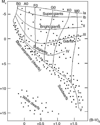
/epubstore/S/P-Schneider/Extragalactic-Astronomy-And-Cosmology/OEBPS/A129044_2_En_BookBackmatter_Fig4_HTML.jpg

Fig. B.2

Schematic color-magnitude diagram in which the spectral types and luminosity classes are indicated. Source: http://de.wikipedia.org

Since stars exist which have, for the same spectral type and hence the same color temperature (and roughly the same effective temperature), very different luminosities, we can deduce immediately that these stars have different radii, as can be read from ( B.2 ). Therefore, stars on the red giant branch, with their much higher luminosities compared to main-sequence stars of the same spectral class, have a much larger radius than the corresponding main-sequence stars. This size effect is also observed spectroscopically: the gravitational acceleration on the surface of a star (surface gravity) is

$\displaystyle{ g = \frac{GM} {R^{2}} \;. }$

(B.3)

We know from models of stellar atmospheres that the width of spectral lines depends on the gravitational acceleration on the star’s surface: the lower the surface gravity, the narrower the stellar absorption lines. Hence, a relation exists between the line width and the stellar radius. Since the radius of a star—for a fixed spectral type or effective temperature—specifies the luminosity, this luminosity can be derived from the width of the lines. In order to calibrate this relation, stars of known distance are required.

Based on the width of spectral lines, stars are classified into luminosity classes : stars of luminosity class I are called supergiants, those of luminosity class III are giants, main-sequence stars are denoted as dwarfs and belong to luminosity class V; in addition, the classification can be further broken down into bright giants (II), subgiants (IV), and subdwarfs (VI). Any star in the Hertzsprung–Russell diagram can be assigned a luminosity class and a spectral class (Fig. B.2 ). The Sun is a G2 star of luminosity class V.

If the distance of a star, and thus its luminosity, is known, and if in addition its surface gravity can be derived from the line width, we obtain the stellar mass from these parameters. By doing so, it turns out that for main-sequence stars the luminosity is a steep function of the stellar mass, approximately described by

$\displaystyle{ \frac{L} {L_{\odot }} \approx \left ( \frac{M} {M_{\odot }}\right )^{3.5}\;. }$

(B.4)

Therefore, a main-sequence star of M = 10 M _⊙ is ∼ 3000 times more luminous than our Sun.

B.3 Structure and evolution of stars

To a very good approximation, stars are spherically symmetric. Therefore, the structure of a star is described by the radial profile of the parameters of its stellar plasma. These are density, pressure, temperature, and chemical composition of the matter. During almost the full lifetime of a star, the plasma is in hydrostatic equilibrium, so that pressure forces and gravitational forces are of equal magnitude and directed in opposite directions, so as to balance each other.

The density and temperature are sufficiently high in the center of a star that thermonuclear reactions are ignited. In main-sequence stars, hydrogen is fused into helium, thus four protons are combined into one ⁴ He nucleus. For every helium nucleus that is produced this way, 26. 73 MeV of energy are released. Part of this energy is emitted in the form of neutrinos which can escape unobstructed from the star due to their very low cross section. ² The energy production rate is approximately proportional to T ⁴ for temperatures below about 15 × 10 ⁶ K, at which the reaction follows the so-called pp-chain. At higher temperatures, another reaction chain starts to contribute, the so-called CNO cycle, with an energy production rate which is much more strongly dependent on temperature—roughly proportional to T ²⁰ .

The energy generated in the interior of a star is transported outwards, where it is then released in the form of electromagnetic radiation. This energy transport may take place in two different ways: first, by radiation transport, and second, it can be transported by macroscopic flows of the stellar plasma. This second mechanism of energy transport is called convection; here, hot elements of the gas rise upwards, driven by buoyancy, and at the same time cool ones sink downwards. The process is similar to that observed in heating water on a stove. Which of the two processes is responsible for the energy transport depends on the temperature profile inside the star. The intervals in a star’s radius in which energy transport takes place via convection are called convection zones. Since in convection zones stellar material is subject to mixing, the chemical composition is homogeneous there. In particular, chemical elements produced by nuclear fusion are transported through the star by convection.

Fig. B.3

Theoretical temperature-luminosity diagram of stars. The solid curve is the zero age main sequence (ZAMS), on which stars ignite the burning of hydrogen in their cores. The evolutionary tracks of these stars are indicated by the various lines which are labeled with the stellar mass. The hatched areas mark phases in which the evolution proceeds only slowly, so that many stars are observed to be in these areas. Source: A. Maeder & G. Meynet 1989, Grids of evolutionary models from 0.85 to 120 solar masses - Observational tests and the mass limits , A&A 210, 155, p. 166, Fig. 15. ©ESO. Reproduced with permission

Stars begin their lives with a homogeneous chemical composition, resulting from the composition of the molecular cloud out of which they are formed. If their mass exceeds about 0. 08 M _⊙ , the temperature and pressure in their core are sufficient to ignite the fusion of hydrogen into helium. Gas spheres with a mass below ∼ 0. 08 M _⊙ will not satisfy these conditions, hence these objects—they are called brown dwarfs—are not stars in a proper sense. ³ At the onset of nuclear fusion, the star is located on the zero-age main sequence (ZAMS) in the HRD (see Fig. B.3 ). The energy production by fusion of hydrogen into helium alters the chemical composition in the stellar interior; the abundance of hydrogen decreases by the same rate as the abundance of helium increases. As a consequence, the duration of this phase of central hydrogen burning is limited. As a rough estimate, the conditions in a star will change noticeably when about 10 % of its hydrogen is used up. Based on this criterion, the lifetime of a star on the main sequence can now be estimated. The total energy produced in this phase can be written as

$\displaystyle{ E_{\mathrm{MS}} = 0.1 \times \mathit{M\,c}^{2} \times 0.007\;, }$

(B.5)

where M c ² is the rest-mass energy of the star, of which a fraction of 0.1 is fused into helium, which is supposed to occur with an efficiency of 0.007. Phrased differently, in the fusion of four protons into one helium nucleus, an energy of ∼ 0. 007 × 4 m _p c ² is generated, with m _p denoting the proton mass. In particular, ( B.5 ) states that the total energy produced during this main-sequence phase is proportional to the mass of the star. In addition, we know from ( B.4 ) that the luminosity is a steep function of the stellar mass. The lifetime of a star on the main sequence can then be estimated by equating the available energy E _MS with the product of luminosity and lifetime. This yields

$\displaystyle{ t_{\mathrm{MS}}=\frac{E_{\mathrm{MS}}} {L} \approx 8\times 10^{9}\frac{M/M_{\odot }} {L/L_{\odot }} \,\mathrm{yr} \approx 8 \times 10^{9}\,\left ( \frac{M} {M_{\odot }}\right )^{-2.5}\,\mathrm{yr}\;. }$

(B.6)

Using this argument, we observe that stars of higher mass conclude their lives on the main sequence much faster than stars of lower mass. The Sun will remain on the main sequence for about eight to ten billion years, with about half of this time being over already. In comparison, very luminous stars, like O and B stars, will have a lifetime on the main sequence of only a few million years before they have exhausted their hydrogen fuel.

In the course of their evolution on the main sequence, stars move away only slightly from the ZAMS in the HRD, towards somewhat higher luminosities and lower effective temperatures. In addition, the massive stars in particular can lose part of their initial mass by stellar winds. The evolution after the main-sequence phase depends on the stellar mass. Stars of very low mass, M ≲ 0. 7 M _⊙ , have a lifetime on the main sequence which is longer than the age of the Universe, therefore they cannot have moved away from the main sequence yet.

For massive stars, M ≳ 2. 5 M _⊙ , central hydrogen burning is first followed by a relatively brief phase in which the fusion of hydrogen into helium takes place in a shell outside the center of the star. During this phase, the star quickly moves to the ‘right’ in the HRD, towards lower temperatures, and thereby expands strongly. After this phase, the density and temperature in the center rise so much as to ignite the fusion of helium into carbon. A central helium-burning zone will then establish itself, in addition to the source in the shell where hydrogen is burned. As soon as the helium in the core has been exhausted, a second shell source will form fusing helium. In this stage, the star will become a red giant or supergiant, ejecting part of its mass into the interstellar medium in the form of stellar winds. Its subsequent evolutionary path depends on this mass loss. A star with an initial mass M ≲ 8 M _⊙ will evolve into a white dwarf, which will be discussed further below.

For stars with initial mass M ≲ 2. 5 M _⊙ , the helium burning in the core occurs explosively, in a so-called helium flash. A large fraction of the stellar mass is ejected in the course of this flash, after which a new stable equilibrium configuration is established, with a helium shell source burning beside the hydrogen-burning shell. Expanding its radius, the star will evolve into a red giant or supergiant and move along the asymptotic giant branch (AGB) in the HRD.

The configuration in the helium shell source is unstable, so that its burning will occur in the form of pulses. After some time, this will lead to the ejection of the outer envelope which then becomes visible as a planetary nebula . The remaining central star moves to the left in the HRD, i.e., its temperature rises considerably (to more than 10 ⁵ K). Finally, its radius gets smaller by several orders of magnitude, so that the stars move downwards in the HRD, thereby slightly reducing its temperature: a white dwarf is born, with a mass of about 0. 6 M _⊙ and a radius roughly corresponding to that of the Earth.

If the initial mass of the star is ≳ 8 M _⊙ , the temperature and density at its center become so large that carbon can also be fused. Subsequent stellar evolution towards a core-collapse supernova is described in Sect. 2.3.2 .

The individual phases of stellar evolution have very different time-scales. As a consequence, stars pass through certain regions in the HRD very quickly, and for this reason stars at those evolutionary stages are never or only rarely found in the HRD. By contrast, long-lasting evolutionary stages like the main sequence or the red giant branch exist, with those regions in an observed HRD being populated by numerous stars.

C: Units and constants

In this book, we consistently used, besides astronomical units, the Gaussian cgs system of units, with lengths measured in cm, masses in g, and energies in erg. This is the commonly used system of units in astronomy. In these units, the speed of light is $c = 2.998 \times 10^{10}\,\mathrm{cm\,s^{-1}}$ , the masses of protons, neutrons, and electrons are $m_{\mathrm{p}} = 1.673 \times 10^{-24}\,\mathrm{g}$ , $m_{\mathrm{n}} = 1.675 \times 10^{-24}\,\mathrm{g}$ , and $m_{\mathrm{e}} = 9.109 \times 10^{-28}\,\mathrm{g}$ , respectively.

Frequently used units of length in astronomy include the Astronomical Unit, thus the average separation between the Earth and the Sun, where 1 AU = 1. 496 × 10 ¹³ cm, and the parsec (see Sect. 2.2.1 for the definition), 1 pc = 3. 086 × 10 ¹⁸ cm. A year has 1 yr = 3. 156 × 10 ⁷ s. In addition, masses are typically specified in Solar masses, 1 M _⊙ = 1. 989 × 10 ³³ g, and the bolometric luminosity of the Sun is $L_{\odot } = 3.846 \times 10^{33}\,\mathrm{erg\,s^{-1}}$ .

In cgs units, the value of the elementary charge is $e = 4.803 \times 10^{-10}\,\mathrm{cm}^{3/2}\,\mathrm{g}^{1/2}\,\mathrm{s}^{-1}$ , and the unit of the magnetic field strength is one Gauss, where $1\,\mathrm{G} = 1\,\mathrm{g}^{1/2}\,\mathrm{cm}^{-1/2}\,\mathrm{s}^{-1} = 1\,\mathrm{erg}^{1/2}\,\mathrm{cm}^{-3/2}$ . One of the very convenient properties of cgs units is that the energy density of the magnetic field in these units is given by $\rho _{B} = B^{2}/(8\pi )$ —the reader may check that the units of this equation are consistent.

X-ray astronomers measure energies in electron Volts, where $1\mathrm{eV} = 1.602 \times 10^{-12}\,\mathrm{erg}$ . Temperatures can also be measured in units of energy, because k _B T has the dimension of energy. They are related according to 1 eV = 1. 161 × 10 ⁴ k _B K. Since we always use the Boltzmann constant k _B in combination with a temperature, its actual value is never needed. The same holds for Newton’s constant of gravity which is always used in combination with a mass. Here one has

$\displaystyle{ \frac{G\,M_{\odot }} {c^{2}} = 1.495 \times 10^{5}\,\mathrm{cm}\;, }$

(C.1)

which can also be written in the form

$\displaystyle{ G = 4.35 \times 10^{-3}\, \frac{\mathrm{pc}} {M_{\odot }}\left (\frac{\mathrm{km}} {s} \right )^{2}\;. }$

(C.2)

The frequency of a photon is linked to its energy according to h _P ν = E , and we have the relation $1\mathrm{eV}\,h_{\mathrm{P}}^{-1} = 2.418 \times 10^{14}\,\mathrm{s}^{-1} = 2.418 \times 10^{14}\,\mathrm{Hz}$ . Accordingly, we can write the wavelength $\lambda = c/\nu = h_{\mathrm{P}}c/E$ in the form

$\displaystyle{ \frac{h_{\mathrm{P}}c} {1\,\mathrm{eV}} = 1.2400 \times 10^{-4}\,\mathrm{cm} = 12\,400\,{\AA}\;.}$

D: Recommended literature

In the following, we will give some recommendations for further study of the literature on astrophysics. For readers who have been in touch with astronomy only occasionally until now, the general textbooks may be of particular interest. The choice of literature presented here is a very subjective one which represents the preferences of the author, and of course it represents only a small selection of the many astronomy texts available.

D.1 General textbooks

There exist a large selection of general textbooks in astronomy which present an overview of the field at a non-technical level. A classic one (though by now becoming of age) and an excellent presentation of astronomy is

F. Shu: The Physical Universe: An Introduction to Astronomy , University Science Books, Sausalito, 1982.

Turning to more technical books, at about the level of the present text, my favorite is

B.W. Carroll & D.A. Ostlie: An Introduction to Modern Astrophysics , Addison-Wesley, Reading, 2006;

its ∼ 1400 pages cover the whole range of astronomy. The texts

M.L. Kutner: Astronomy: A physical perspective , Cambridge University Press, Cambridge, 2003,
J.O. Bennett, M.O. Donahue, N. Schneider & M. Voit: The Cosmic Perspective , Addison-Wesley, 2013,

also cover the whole field of astronomy. A text with a particular focus on stellar and Galactic astronomy is

A. Unsöld & B. Baschek: The New Cosmos , Springer-Verlag, Berlin, 2002;

The book

M.H. Jones & R.J.A. Lambourne: An Introduction to Galaxies and Cosmology , Cambridge University Press, Cambridge, 2003

covers the topics described in this book and is also highly recommended; it is less technical than the present text.

D.2 More specific literature

More specific monographs and textbooks exist for the individual topics covered in this book, some of which shall be suggested below. Again, this is just a brief selection. The technical level varies substantially among these books and, in general, exceeds that of the present text.

Astrophysical processes:

M. Harwit: Astrophysical Concepts , Springer, New-York, 2006,
G.B. Rybicki & A.P. Lightman: Radiative Processes in Astrophysics , John Wiley & Sons, New York, 1979,
F. Shu: The Physics of Astrophysics I: Radiation , University Science Books, Mill Valley, 1991,
F. Shu: The Physics of Astrophysics II: Gas Dynamics , University Science Books, Mill Valley, 1991,
S.N. Shore: The Tapestry of Modern Astrophysics , Wiley-VCH, Berlin, 2002,
D.E. Osterbrock & G.J. Ferland: Astrophysics of Gaseous Nebulae and Active Galactic Nuclei , University Science Books, Mill Valley, 2005.

Furthermore, there is a three-volume set of books,

T. Padmanabhan: Theoretical Astrophysics: I. Astrophysical Processes. II. Stars and Stellar Systems. III. Galaxies and Cosmology , Cambridge University Press, Cambridge, 2000.

Galaxies and gravitational lenses:

L.S. Sparke & J.S. Gallagher: Galaxies in the Universe: An Introduction , Cambridge University Press, Cambridge, 2007,
J. Binney & M. Merrifield: Galactic Astronomy , Princeton University Press, Princeton, 1998,
J. Binney & S. Tremaine: Galactic dynamics , Princeton University Press, Princeton, 2008,
R.C. Kennicutt, Jr., F. Schweizer & J.E. Barnes: Galaxies: Interactions and Induced Star Formation , Saas-Fee Advanced Course 26, Springer-Verlag, Berlin, 1998,
B.E.J. Pagel: Nucleosynthesis and Chemical Evolution of Galaxies , Cambridge University Press, Cambridge, 2009,
F. Combes, P. Boissé, A. Mazure & A. Blanchard: Galaxies and Cosmology , Springer-Verlag, 2004,
P. Schneider, J. Ehlers & E.E. Falco: Gravitational Lenses , Springer-Verlag, New York, 1992.
P. Schneider, C.S. Kochanek & J. Wambsganss: Gravitational Lensing: Strong, Weak & Micro , Saas-Fee Advanced Course 33, G. Meylan, P. Jetzer & P. North (Eds.), Springer-Verlag, Berlin, 2006.

Active galaxies:

B.M. Peterson: An Introduction to Active Galactic Nuclei , Cambridge University Press, Cambridge, 1997,
R.D. Blandford, H. Netzer & L. Woltjer: Active Galactic Nuclei , Saas-Fee Advanced Course 20, Springer-Verlag, 1990,
J. Krolik: Active Galactic Nuclei , Princeton University Press, Princeton, 1999,
J. Frank, A. King & D. Raine: Accretion Power in Astrophysics , Cambridge University Press, Cambridge, 2012.

Cosmology:

M.S. Longair: Galaxy Formation , Springer-Verlag, Berlin, 2008,
J.A. Peacock: Cosmological Physics , Cambridge University Press, Cambridge, 1999,
T. Padmanabhan: Structure formation in the Universe , Cambridge University Press, Cambridge, 1993,
E.W. Kolb and M.S. Turner: The Early Universe , Addison Wesley, 1990,
S. Dodelson: Modern Cosmology , Academic Press, San Diego, 2003,
P.J.E. Peebles: Principles of Physical Cosmology , Princeton University Press, Princeton, 1993,
G. Börner: The Early Universe , Springer-Verlag, Berlin, 2003,
D.H. Lyth & A.R. Liddle: The Primordial Density Perturbation: Cosmology, Inflation and the Origin of Structure , Cambridge University Press, Cambridge, 2009.

D.3 Review articles, current literature, and journals

Besides textbooks and monographs, review articles on specific topics are particularly useful for getting extended information about a special field. A number of journals and series exist in which excellent review articles are published. Among these are Annual Reviews of Astronomy and Astrophysics (ARA&A) and Astronomy & Astrophysics Reviews (A&AR), both publishing astronomical articles only. In Physics Reports (Phys. Rep.) and Reviews of Modern Physics (RMP), astronomical review articles are also frequently found. Such articles are also published in the lecture notes of international summer/winter schools and in the proceedings of conferences; of particular note are the Lecture Notes of the Saas-Fee Advanced Courses . A very useful archive containing review articles on the topics covered in this book is the Knowledgebase for Extragalactic Astronomy and Cosmology, which can be found at

http://nedwww.ipac.caltech.edu/level5 .

Original astronomical research articles are published in the relevant scientific journals; most of the figures presented in this book are taken from these journals. The most important of them are Astronomy & Astrophysics (A&A), The Astronomical Journal (AJ), The Astrophysical Journal (ApJ), Monthly Notices of the Royal Astronomical Society (MNRAS), and Publications of the Astronomical Society of the Pacific (PASP). Besides these, a number of smaller, regional, or more specialized journals exist, such as Astronomische Nachrichten (AN), Acta Astronomica (AcA), or Publications of the Astronomical Society of Japan (PASJ). Some astronomical articles are also published in the journals Nature and Science. The Physical Review D and Physical Review Letters contain an increasing number of papers on astrophysical cosmology.

Since many years now, the primary source of astronomical information by far is the electronic archive

http://arxiv.org/archive/astro-ph

which is freely accessible. This archive, now hosted at Cornell University and supported by the Simons Foundation and the Allianz der deutschen Wissenschaftsorganisationen, koordiniert durch TIB, MPG und HGF, has existed since 1992, with an increasing number of articles being stored at this location. In particular, in the fields of extragalactic astronomy and cosmology, almost all articles that are published in the major journals can be found in this archive. A large number of review articles and coference proceedings are also available here.

The SAO/NASA Astrophysics Data System (ADS) is a Digital Library portal for Astronomy and Physics, operated by the Smithsonian Astrophysical Observatory (SAO) under a NASA grant. It can be accessed via the Internet at, e.g.,

http://cdsads.u-strasbg.fr/abstract_service.html ,

http://adsabs.harvard.edu/abstract_service.html ,

and it provides the best access to astronomical literature. Besides tools to search for authors and keywords, ADS offers also direct access to older articles that have been scanned. The access to more recent articles, and to all articles in some other journals, is restricted to IP addresses that are associated with a subscription for the respective journals—but ADS also contains a link to the article in the arXiv (if it has been posted there), so also these articles are accessible.

E: Acronyms used

In this Appendix, we compile some of the acronyms that are used, and references to the sections in which these acronyms have been introduces or explained.

2dF(GRS)	–2 degree Field Galaxy Redshift Survey (Sect. 8.1.2 )
2MASS	–Two Micron All Sky Survey (Sect. 1.4 )
AAS	–American Astronomical Society
AAT	–Anglo-Australian Telescope (Sect. 1.3.3 )
ACBAR	–Arcminute Cosmology Bolometer Array
	–Receiver (Sect. 8.6.5 )
ACO	–Abell, Corwin & Olowin (catalogue of clusters of galaxies, Sect. 6.2.1 )
ACS	–Advanced Camera for Surveys (HST instrument—Sect. 1.3.3 )
ACT	–Atacama Cosmology Telescope (Sect. 8.6.6 )
ADAF	–Advection-Dominated Accretion Flow (Sect. 5.3.2 )
AGB	–Asymptotic Giant Branch (Sect. 3.5.2 )
AGN	–Active Galactic Nucleus (Sect. 5)
ALMA	–Atacama Large Millimeter/sub-millimeter Array (Sect. 1.3.1 )
AMR	–Adaptive Mesh Refinement (Sect. 10.6.1 )
APEX	–Atacama Pathfinder Experiment (Sect. 1.3.1 )
ASP	–Astronomical Society of the Pacific
AU	–Astronomical Unit
BAL	–Broad Absorption Line (-Quasar, Sect. 5.7 )
BAOs	–Baryonic Acoustic Oscillations (Sect. 7.4.3 )
BATSE	–Burst And Transient Source Experiment (CGRO instrument, Sect. 9.7 )
BBB	–Big Blue Bump (Sect. 5.4.1 )
BBN	–Big Bang Nucleosynthesis (Sect. 4.4.5 )
BCD	–Blue Compact Dwarf (Sect. 3.2.1 )
BCG	–Brightest Cluster Galaxy (Sect. 6.2.4 )
BH	–Black Hole (Sect. 5.3.5 )
BLR	–Broad Line Region (Sect. 5.4.2 )
BLRG	–Broad Line Radio Galaxy (Sect. 5.2.4 )
BOOMERANG	–Balloon Observations Of Millimetric Extragalactic Radiation and Geophysics (Sect. 8.6.4 )
BTP diagram	–Baldwin–Phillips–Terlevich diagram (Sect. 5.4.3 )
CBI	–Cosmic Background Imager (Sect. 8.6.5 )
CCAT	–Cerro Chajnantor Atacama Telescope (Chap. 11 )
CCD	–Charge Coupled Device
CDF	–Chandra Deep Field (Sect. 9.2.1 )
CDM	–Cold Dark Matter (Sect. 7.4.1 )
CERN	–Conseil European pour la Recherché Nucleaire
CfA	–Harvard-Smithsonian Center for Astrophysics
CFHT	–Canada-France-Hawaii Telescope (Sect. 1.3.3 )
CFRS	–Canada-France Redshift Survey (Sect. 8.1.2 )
COSMOS	–Cosmological Evolution Survey (Sect. 9.2.1 )
CTIO	–Cerro Tololo Inter-American Observatory
CXB	–Cosmic X-ray Background (Sect. 9.5.3 )
DASI	–Degree Angular Scale Interferometer (Sect. 8.6.4 )
DES	–Dark Energy Survey (Chap. 11 )
DIRBE	–Diffuse Infrared Background Experiment (instrument onboard COBE)
DLA system	–Damped Lyman Alpha system (Sect. 9.3.4 )
DRG	–Distant Red Galaxy (Sect 9.1.3)
dSph	–dwarf Spheroidal (Sect. 3.2.1 )
DSS	–Digital Sky Survey (Sect. 1.4 )
ECDFS	–Extended Chandra Deep Field South (Sect. 9.3.3 )
EdS	–Einstein–de Sitter (Sect. 4.3.4 )
E-ELT	–European Extremely Large Telescope (Chap. 11 )
EMSS	–Extended Medium Sensitivity Survey (Sect. 6.4 .5)
EPIC	–European Photon Imaging Camera (XMM-Newton instrument)
ERO	–Extremely Red Object (Sect. 9.3.2 )
EROS	–Expérience pour la Recherche d’Objets Sombres (microlensing collaboration, Sect. 2.5 )
ESA	–European Space Agency
ESO	–European Southern Observatory
FFT	–Fast Fourier Transform (Sect. 7.5.3 )
FIR	–Far Infrared
FIRAS	–Far Infrared Absolute Spectrophotometer (instrument onboard COBE; see Fig. 4.3 )
FJ	–Faber–Jackson (Sect. 3.4.2 )
FOC	–Faint Object Camera (HST instrument)
FORS	–Focal Reducer / Low Dispersion Spectrograph (VLT instrument)
FOS	–Faint Object Spectrograph (HST instrument)
FP	–Fundamental Plane (Sect. 3.4.3 )
FR (I/II)	–Fanaroff–Riley Type (Sect. 5.1.2 )
FUSE	–Far Ultraviolet Spectroscopic Explorer (Sect. 1.3.4 )
FWHM	–Full Width Half Maximum (Sect. 5.1.4 )
GALEX	–Galaxy Evolution Explorer (Sect. 1.3.4 )
GBM	–Gamma-ray Burst Monitor (instrument on Fermi—Sect. 1.3.6 )
GC	–Galactic Center (Sects. 2.3 , 2.6)
GEMS	–Galaxy Evolution from Morphology and Spectral Energy Distributions (Sect. 9.2.1 )
GGL	–Galaxy-Galaxy Lensing (Sect. 7.7 )
GMT	–Giant Magellan Telescope (Chap. 11 )
GOODS	–Great Observatories Origins Deep Survey (Sect. 9.2.1 )
GR	–General Relativity
GRB	–Gamma-Ray Burst (Sect. 1.3.5 , 9.7)
GTC	–Gran Telescopio Canarias (Sect. 1.3.3 )
GUT	–Grand Unified Theory (Sect. 4.5.3 )
Gyr	–Gigayear = 10 ⁹ years
GZK	–Greisen–Zatsepin–Kuzmin (Sect. 2.3.4 )
HB	–Horizontal Branch
HCG	–Hickson Compact Group (catalogue of galaxy groups, Sect. 6.2.3 )
HDF(N/S)	–Hubble Deep Field (North/South) (Sect. 1.3.3 , 9.2.1)
HDM	–Hot Dark Matter (Sect. 7.4.1 )
HEAO	–High Energy Astrophysical Observatory (Sect. 1.3.5 )
H.E.S.S.	–High Energy Stereoscopic System (Sect. 1.3.6 )
HFI	–High-Frequency Instrument (onboard the Planck satellite; Sect. 8.6.6 )
HIFI	–Heterodyne Instrument for the Far Infrared (Herschel instrument—Sect. 1.3.2 )
HLS	–Herschel Lensing Survey (Sect. 9.2.3 )
HRD	–Hertzsprung–Russell Diagram (Appendix A.4.4 )
HRI	–High Resolution Imager (ROSAT instrument)
HST	–Hubble Space Telescope (Sect. 1.3.3 )
HVC	–High Velocity Cloud (Sect. 2.3.6 )
HUDF	–Hubble Ultradeep Survey (Sect. 9.2.1 )
IAU	–International Astronomical Union
ICL	–IntraCluster Light (Sect. 6.3.4 )
ICM	–Intra-Cluster Medium (Chap. 6 )
IFU	–Integral Field Unit (Sect. 1.3.3 )
IGM	–Intergalactic Medium (Sect. 10.3 )
IMF	–Initial Mass Function (Sect. 3.5.1 )
IoA	–Institute of Astronomy (Cambridge)
IR	–Infrared (Sect. 1.3.2 )
IRAC	–Infrared Array Camera (instrument on Spitzer—Sect. 1.3.2 )
IRAS	–Infrared Astronomical Observatory (Sect. 1.3.2 )
IRS	–Infrared Spectrograph (instrument on Spitzer—Sect. 1.3.2 )
ISM	–Interstellar Medium
ISO	–Infrared Space Observatory (Sect. 1.3.2 )
ISW effect	–Integrated Sachs–Wolfe effect (Sect. 8.6.1 )
IUE	–International Ultraviolet Explorer (Sect. 1.3.4 )
IVC	–Intermediate-Velocity Cloud (Sect. 2.3.7 )
JCMT	–James Clerk Maxwell Telescope (Sect. 1.3.1 )
JVAS	–Jodrell Bank-VLA Astrometric Survey (Sect. 3.11.3 )
JWST	–James Webb Space Telescope (Chap. 11 )
KAO	–Kuiper Airborne Observatory (Sect. 1.3.2 )
KiDS	–KiLO Degree Survey (Chap. 11 )
LAB	–Leiden-Argentine-Bonn (Sect. 1.4 )
LAE	–Lyman Alpha Emitter (Sect 9.1.3)
LAT	–Large Area Telescope (instrument on Fermi—Sect. 1.3.6 )
LBG	–Lyman-Break Galaxy (Sect. 9.1.1 )
LBT	–Large Binocular Telescope (Sect. 1.3.3 )
LCRS	–Las Campanas Redshift Survey (Sect. 8.1.2 )
LFI	–Low-Frequency Instrument (onboard the Planck satellite; Sect. 8.6.6 )
LHC	–Large Hadron Collider
LINER	–Low-Ionization Nuclear Emission-Line Region (Sect. 5.2.3 )
LIRG	–Luminous InfraRed Galaxy (Sect. 9.4.1 )
LISA	–Laser Interferometer Space Antenna (Chap. 11 )
LMC	–Large Magellanic Cloud
LMT	–Large Millimeter Telescope (Chap. 11 )
LOFAR	–Low Frequency Array (Chap. 11 )
LSB galaxy	–Low Surface Brightness galaxy (Sect. 3.3.2 )
LSR	–Local Standard of Rest (Sect. 2.4.1 )
LSS	–Large-Scale Structure (Chap. 8 )
LSST	–Large Synoptic Survey Telescope (Chap. 11 )
MACHO	–Massive Compact Halo Object (and collaboration of the same name, Sect. 2.5 )
MAGIC	–Major Atmospheric Gamma-ray Imaging Cherenkov telescope (Sect. 1.3.6 )
MAMBO	–Max-Planck Millimeter Bolometer (Sect. 9.3.3 )
MAXIMA	–Millimeter Anisotropy Experiment Imaging Array (Sect. 8.6.4 )
MDM	–Mixed Dark Matter (Sect. 7.4.2 )
MIPS	–Multiband Imaging Photometer for Spitzer (instrument on Spitzer— Sect. 1.3.2 )
MIR	–Mid-Infrared
MLCS	–Multi-Color Light Curve Shape (Sect. 3.9.4 )
MMT	–Multi-Mirror Telescope
MOND	–Modified Newtonian Dynamics (Chap. 11 )
MS	–used for the ‘Main Sequence’ of stars, or the ‘Millennium Simulation’ (Sect. 7.5.3 )
MW	–Milky Way
MXXL	–Millennium XXL simulation (Sect. 7.5.3 )
NAOJ	–National Astronomical Observatory of Japan
NFW	–Navarro, Frenk & White (-profile, Sect. 7.6.1 )
NGC	–New General Catalog (Chap. 3 )
NGP	–North Galactic Pole (Sect. 2.1 )
NICMOS	–Near Infrared Camera and Multi-Object Spectrometer (HST instrument— Sect. 1.3.3 )
NIR	–Near Infrared
NLR	–Narrow Line Region (Sect. 5.4.3 )
NLRG	–Narrow Line Radio Galaxy (Sect. 5.2.4 )
NOAO	–National Optical Astronomy Observatory
NRAO	–National Radio Astronomy Observatory
NTT	–New Technology Telescope (Sect. 1.3.3 )
NVSS	–NRAO VLA Sky Survey (Sect. 1.4 )
OGLE	–Optical Gravitational Lensing Experiment (microlensing collaboration, Sect. 2.5 )
OVV	–Optically Violently Variable (Sect. 5.2.5 )
PACS	–Photodetector Array Camera and Spectrometer (Herschel instrument— Sect. 1.3.2 )
PL	–Period-Luminosity (Sect. 2.2.7 )
PLANET	–Probing Lensing Anomalies Network (microlensing collaboration, Sect. 2.5 )
PM	–Particle-Mesh (Sect. 7.5.3 )
P ³ M	–Particle-Particle Particle-Mesh (Sect. 7.5.3 )
PN	–Planetary Nebula
POSS	–Palomar Observatory Sky Survey (Sect. 1.4 )
PSF	–Point Spread Function
PSPC	–Position-Sensitive Proportional Counter (ROSAT instrument)
QCD	–Quantum Chromodynamics (Sect. 4.4.1 )
QSO	–Quasi-Stellar Object (Sect. 5.2.1 )
RASS	–ROSAT All-Sky Survey (Sect. 6.4 .5)
RCS	–Red Cluster Sequence (Sect. 6.8 )
REFLEX	–ROSAT-ESO Flux-Limited X-Ray survey
RGB	–Red Giant Branch (Sect. 3.5.2 )
ROSAT	–Roentgen Satellite (Sect. 1.3.5 )
SAO	–Smithsonian Astrophysical Observatory
SCUBA	–Sub-millimeter Common-User Bolometer Array (Sect. 1.3.1 )
SDSS	–Sloan Digital Sky Survey (Sects. 1.4 , 8.1.2)
SFR	–Star Formation Rate (Sect. 9.6.1 )
SGP	–South Galactic Pole (Sect. 2.1 )
SIS	–Singular Isothermal Sphere (Sect. 3.11.2 )
SKA	–Square Kilometer Array (Chap. 11 )
SLACS	–Sloan Lens Advanced Camera for Surveys (Sect. 3.11.3 )
SMBH	–Supermassive Black Hole (Sect. 5.3 )
SMC	–Small Magellanic Cloud
SMG	–Sub-Millimeter Galaxy (Sect. 9.3.3 )
SN(e)	–Supernova(e) (Sect. 2.3.2 )
SNR	–Supernova Remnant
SOFIA	–Stratospheric Observatory for Infrared Astronomy (Sect. 1.3.2 )
SPH	–Smooth Particle Hydrodynamics (Sect. 10.6.1 )
SPIRE	–Spectral and Photometric Imaging REceiver (Herschel instrument— Sect. 1.3.2 )
SPT	–South Pole Telescope (Sect. 1.3.1 )
SQLS	–SDSS Quasar Lens Search (Sect. 3.11.3 )
STIS	–Space Telescope Imaging Spectrograph (HST instrument)
STScI	–Space Telescope Science Institute (Sect. 1.3.3 )
SZ	–Sunyaev–Zeldovich (-effect, Sect. 6.4 .4)
TDE	–Tidal Disruption Event (Sect. 5.5.6 )
TeVeS	–Tensor-Vector-Scalar (Chap. 11 )
TF	–Tully–Fisher (Sect. 3.4 )
TMT	–Thirty Meter Telescope (Chap. 11 )
TP-AGB star	–Thermally Pulsating AGB star (Sect. 3.5.5 )
UDF	–Ultra Deep Field (Sect. 9.2.1 )
UHECRs	–Ultra-High Energy Cosmic Rays (Sect. 2.3.4 )
ULIRG	–Ultraluminous Infrared Galaxy (Sect. 9.3.1 )
ULX	–Ultraluminous Compact X-ray Source (Sect. 9.3.1 )
UV	–Ultraviolet
VISTA	–Visible and Infrared Survey Telescope (Sect. 1.3.3 )
VLA	–Very Large Array (Sect. 1.3.1 )
VLBA	–Very Long Baseline Array (Sect. 1.3.1 )
VLBI	–Very Long Baseline Interferometer (Sect. 1.3.1 )
VLT	–Very Large Telescope (Sect. 1.3.3 )
VST	–VLT Survey Telescope (Sect. 1.3.3 )
VVDS	–VIMOS VLT Deep Survey (Sect. 8.1.2 )
WD	–White Dwarf (Sect. 2.3.2 )
WDM	–Warm Dark Matter (Sect. 7.8 )
WFIRST	–Wide Field Infrared Space Telescope (Chap. 11 )
WIMP	–Weakly Interacting Massive Particle (Sect. 4.4.3 )
WISE	–Wide-field Infrared Survey Explorer(Sect. 1.3.2 )
WFC3	–Wide Field Camera 3 (HST instrument—Sect. 1.3.3 )
WFI	–Wide Field Imager (camera at the ESO/MPG 2.2m telescope, La Silla, Sect. 6.6.2 )
WFPC2	–Wide Field and Planetary Camera 2 (HST instrument– Sect. 1.3.3 )
WMAP	–Wilkinson Microwave Anisotropy Probe (Sect. 8.6.5 )
XDF	–eXtremely Deep Field (Sect. 9.2.1 )
XMM	–X-ray Multi-Mirror Mission (Sect. 1.3.5 )
XRB	–X-Ray Background (Sect. 9.5.3 )
ZAMS	–Zero Age Main Sequence (Sect. 3.5.2 )

F: Solutions to problems

Solution to 1.1. If the object at current distance D had a constant velocity v = H ₀ D for all times, it needed a time $t = D/v = 1/H_{0}$ to reach separation D . This time is independent of D . Using ( 1.7 ), we find that

$\displaystyle{H_{0}^{-1} = \frac{3.086 \times 10^{24}\,\mathrm{cm}} {h\,10^{7}\,\mathrm{cm}} \,\mathrm{s} = 9.77\,h^{-1} \times 10^{9}\,\mathrm{yr}\;,}$

where we used that 1 yr = 3. 16 × 10 ⁷ s. For a value of h ≈ 0. 71, this time is comparable to, but slightly larger than the age of the oldest stars. Light can propagate a distance c ∕ H ₀ over the time-scale H ₀ ⁻¹ , where

$\displaystyle{ \frac{c} {H_{0}} = \frac{2.998 \times 10^{5}\,\mathrm{km\;s^{-1}}} {100h\,\mathrm{km\;s^{-1}\,Mpc^{-1}}} = 2.998h^{-1}\,\mathrm{Gpc}\;.}$

Solution to 1.2. The number of galaxies in a sphere of radius $r_{0} = 1\,h^{-1}\,\mathrm{Gpc}$ is $N = (4\pi /3)r_{0}^{3}\,n_{0}$ , where $n_{0} = 2 \times 10^{-2}\,h^{3}\,\mathrm{Mpc}^{-3}$ . Thus,

$\displaystyle\begin{array}{rcl} N& =& (4\pi /3)h^{-3}\,\mathrm{Gpc}^{3}\,2 \times 10^{-2}\,h^{3}\,\mathrm{Mpc}^{-3} {}\\ & =& (8\pi /3)\,10^{7} \approx 8 \times 10^{7}\;. {}\\ \end{array}$

The number of these galaxies per square degree on the sky is obtained by dividing N by the solid angle of the sky, which is 4 π steradian. Since 180 ^∘ corresponds to π rad, we have that $1\,\mathrm{steradian} = (180/\pi )^{2}\,\mathrm{deg}^{2}$ , so that the full sky has a solid angle of $4\pi \,(180/\pi )^{2}\,\mathrm{deg}^{2} = 41253\,\mathrm{deg}^{2}$ . This yields a number density of ∼ 2 × 10 ³ deg ⁻² .

To calculate the fraction of the sky covered by the luminous region of these galaxies, we consider first a thin spherical shell of radius r and thickness d r around us. In this shell, there are d N = 4 π r ² n ₀ d r galaxies, each of them subtending a solid angle of π R ² ∕ r ² , where R = 10 kpc is the radius of the luminous region. Thus, the solid angle covered by all galaxies in the shell is d ω = 4 π ² R ² n ₀ d r . The solid angle covered by all galaxies within distance r ₀ is obtained by integrating this expression over r ,

$\displaystyle{\omega =\int _{ 0}^{r_{0} }\mathrm{d}\omega = 4\pi ^{2}\,R^{2}\,n_{ 0}\int _{0}^{r_{0} }\mathrm{d}r = 4\pi ^{2}\,R^{2}\,n_{ 0}\,r_{0}\;.}$

The fraction of the sky covered by these galaxies is $f =\omega /(4\pi ) =\pi \, R^{2}\,n_{0}\,r_{0} \approx 0.6\,\%$ .

Solution to 1.3.

(1)

The mean baryon density of the Universe is $\rho _{\mathrm{b}} = 0.15\varOmega _{\mathrm{m}}\,3H_{0}^{2}/(8\pi G)$ . Making use of ( 1.14 ), this yields $\rho _{\mathrm{b}} = 4.3 \times 10^{-31}\,\mathrm{g\,cm^{-3}}$ . The estimate to the local mass density yields $\rho _{{\ast}\mathrm{local}} = 1\,M_{\odot }\,\mathrm{pc^{-3}} \approx 2\times 10^{33}\,\mathrm{g}\,(3\times 10^{18}\,\mathrm{cm})^{-3} = (2/27)\times 10^{-21}\,\mathrm{g/cm^{3}} \approx 7\times 10^{-23}\,\mathrm{g/cm^{3}}$ . Thus, ρ _∗local ∕ ρ _b ≈ 1. 6 × 10 ⁸ .

(2)

According to ( 1.1 ), the mass of the Galaxy inside R ₀ is $M = R_{0}\,V _{0}^{2}/G$ , yielding a mean density within R ₀ of

$\displaystyle{\rho _{8} = \frac{M} {(4\pi /3)\,R_{0}^{3}} = \frac{V _{0}^{2}} {(4\pi /3)\,G\,R_{0}^{2}}\;.}$

The mean matter density of the Universe is $\rho _{\mathrm{m}} =\varOmega _{\mathrm{m}}\,3H_{0}^{2}/(8\pi G)$ . With Ω _m ≈ 0. 3, this yields

$\displaystyle\begin{array}{rcl} \frac{\rho _{8}} {\rho _{\mathrm{m}}}& =& \frac{V _{0}^{2}} {(4\pi /3)\,G\,R_{0}^{2}}\, \frac{8\pi G} {\varOmega _{\mathrm{m}}\,3H_{0}^{2}} = \frac{2V _{0}^{2}} {\varOmega _{\mathrm{m}}\,R_{0}^{2}\,H_{0}^{2}} {}\\ & =& \frac{2} {h^{2}\,\varOmega _{\mathrm{m}}}\left ( \frac{220\,\mathrm{km/s}} {8\,\mathrm{kpc}\;100\,\mathrm{(km/s)\,Mpc^{-1}}}\right )^{2} {}\\ & =& \frac{2} {h^{2}\,\varOmega _{\mathrm{m}}}\,\left (0.275 \times 10^{3}\right )^{2} \approx 1.0 \times 10^{6}\;. {}\\ \end{array}$

(3)

The mean number of baryons N _b in the box is the volume of the box times the mean number density of baryons. The latter is given by the mean mass density ρ _b of baryons in the Universe, divided by the mass per baryon, which is m _b ≈ 1. 7 × 10 ⁻²⁴ g. Thus, making use of value of ρ _b derived above,

$\displaystyle\begin{array}{rcl} N_{\mathrm{b}}& \approx & 1\,\mathrm{m}^{3}\,4.3 \times 10^{-31}\,\mathrm{g/cm^{3}}\,(1.7 \times 10^{-24}\,\mathrm{g})^{-1} {}\\ & \approx & (0.43/1.7) \approx 0.25\;. {}\\ \end{array}$

Thus, the mean baryon density in the Universe is about $(1/4)\,\mathrm{m}^{-3}$ .

Solution to 1.4.

(1)

Differentiating the ansatz for r ( t ), one finds $\dot{r} = -\alpha (r_{0}/t_{\mathrm{f}})\left (1 - t/t_{\mathrm{f}}\right )^{\alpha -1}$ , and $\ddot{r} =\alpha (\alpha -1)(r_{0}/t_{\mathrm{f}}^{2})$ $\left (1 - t/t_{\mathrm{f}}\right )^{\alpha -2}$ . Inserting this into the equation of motion yields

$\displaystyle{\alpha (\alpha -1)(r_{0}/t_{\mathrm{f}}^{2})\left (1 - t/t_{\mathrm{ f}}\right )^{\alpha -2} = -GMr_{ 0}^{-2}\left (1-t/t_{\mathrm{ f}}\right )^{-2\alpha }.}$

The powers of the time-dependent term must be the same one both sides, yielding α − 2 = −2 α , or α = 2∕3. Equating the prefactors then yields

$\displaystyle{ \frac{2r_{0}} {9t_{\mathrm{f}}^{2}} = \frac{GM} {r_{0}^{2}} \; \Rightarrow \; t_{\mathrm{f}} = \sqrt{ \frac{2r_{0 }^{3 }} {9GM}}\;.}$

The solution r ( t ) has infinite radius for t → − ∞ , but the inflow velocity $\dot{r}$ tends to zero as t → − ∞ . At t = 0, r (0) = r ₀ , but the velocity $\dot{r}(0)$ is finite and determined by M and r ₀ . For t = t _f , the radius shrinks to zero.

(2)

Replacing the mass by the mean initial density $\bar{\rho }$ of the sphere leads to

$\displaystyle{t_{\mathrm{f}} = \sqrt{ \frac{1} {6\pi G\bar{\rho }}}\;,}$

so that the time-scale t _f depends only on the initial density. We can now compare t _f to the orbital time t _orb = 2 π R ₀ ∕ V ₀ . Using ( 1.1 ), and replacing M by the mean density, we get $t_{\mathrm{orb}} = \sqrt{3\pi /(G\bar{\rho })}$ . Hence, $t_{\mathrm{f}}/t_{\mathrm{orb}} = 1/(\sqrt{18}\pi ) \approx 0.075$ . Thus, t _f ≈ 1. 75 × 10 ⁷ yr.

(3)

Using the mean matter density of the Universe, $\bar{\rho }=\rho _{\mathrm{m}}$ , as given by ( 1.10 ), we obtain

$\displaystyle{t_{\mathrm{f}} = \frac{2} {3\sqrt{\varOmega _{\mathrm{m}}}H_{0}}\;.}$

Hence, t _f is very similar to the estimated age of the Universe, H ₀ ⁻¹ , and agrees with the age of the Einstein–de Sitter model ( 1.13 ), for which Ω _m = 1. Indeed, the expansion history of the Einstein–de Sitter model follows exactly the same equation of motion, except that the relevant solution is an expanding one, r ( t ) ∝ t ^2∕3 , which is obtained from our infalling solution by inverting the arrow of time (note that the equation of motion is invariant against t → − t ), and shifting the origin of the time axis.

Solution to 2.1. The angular diameter is δ = 3476∕385000 ≈ 9. 03 × 10 ⁻³ . To convert this to degrees, we recall that π = 180 ^∘ , so that $\delta \approx 9.03 \times 10^{-3}\,(180^{\circ }/\pi ) \approx 0.517^{\circ }\approx 31^{{\prime}}$ . The solid angle covered by the Moon is (0. 517 ^∘ ) ² π ∕4 ≈ 0. 21 deg ² , so the fraction it covers of the full sky is (cf. problem 1.2) 0. 21∕41253 ≈ 5. 1 × 10 ⁻⁶ .

Solution to 2.2. The total energy radiated throughout the galaxy’s lifetime is E = L t , where t = 10 ¹⁰ yr is the assumed age. The energy generated is the mass that is converted into helium in nuclear fusion, times the energy released per unit mass. The former is Y M , where Y is the helium mass fraction generated by nuclear fusion. The energy released per unit mass is ε c ² , where ε is the efficiency of this energy generating process, given by the ratio of the binding energy per nucleon in helium ( ∼ 28 MeV∕4 = 7 MeV) and the mass per nucleon, m _nuc ≈ m _p ≈ 938 MeV; i.e., ε ≈ 0. 008. Thus, the total energy released is E = M Y ε c ² . Equating this to L t , we obtain

$\displaystyle{Y = \frac{L\,t} {\epsilon \,M\,c^{2}} = \frac{1} {3\epsilon }\, \frac{L_{\odot }\,t} {M_{\odot }\,c^{2}}\;,}$

where we used the mass-to-light ratio. Inserting the values for M _⊙ ≈ 2 × 10 ³³ g and L _⊙ ≈ 3. 8 × 10 ³³ erg∕s, and using t ≈ 3. 1 × 10 ¹⁷ s, we obtain Y ≈ 2. 7 % . This value is lower by a factor of ten than the observed helium abundance. On the other hand, adding this value to the helium abundance from BBN yields a result which is very close to the currently observed helium abundance in local galaxies.

Solution to 2.3. According to the Kepler rotation, $V (R) = \sqrt{G\,M(R)/R}$ , a constant V implies M ( R ) ∝ R . The relation between M and ρ is

$\displaystyle{M(R) = 4\pi \int _{0}^{R}\mathrm{d}r\;r^{2}\,\rho (r)\;.}$

Differentiating this w.r.t. R yields $\mathrm{d}M/\mathrm{d}R = 4\pi \,R^{2}\,\rho (R)$ . On the other hand, M ( R ) ∝ R implies $\mathrm{d}M/\mathrm{d}R =\mathrm{ const.}$ , so that ρ ( r ) r ² = const., or ρ ( r ) ∝ r ⁻² .

Solution to 2.4. Light at the Solar limb is deflected by $\hat{\alpha }_{\odot } = 1.\!\!^{{\prime\prime}}74$ , which is far smaller than the angular radius θ _⊙ = 16 ^′ of the Sun. Hence, if we consider a cone of light rays with vertex at the Earth and an opening angle of θ _⊙ , this cone will continue to diverge after being deflected at the Solar limb. If the Sun had a larger distance D , its angular radius would be smaller, namely $\theta = (D/1\,\mathrm{AU})^{-1}\theta _{\odot }$ . If θ equals $\hat{\alpha }_{\odot }$ , the rays of the cone with opening angle θ at Earth would be parallel after light deflection at the Solar limb, and if the distance was slightly larger they would converge after deflection and go through a common focus. If a source was placed at this focus, the Sun would then produce an Einstein ring. Displacing the source slightly, the ring breaks up into a pair of images, with angular separation 2 θ . Thus, the minimum distance for lensing is $D =\theta _{\odot }/\hat{\alpha }_{\odot }\ \mathrm{AU} \approx 552\,\mathrm{AU}$ , and the image splitting at the minimum distance would be $2\hat{\alpha }_{\odot }\approx 3.\!\!^{{\prime\prime}}48$ .

Solution to 2.5. Kepler rotation yields $V (r) = \sqrt{GM_{\bullet } /r}$ , which we rewrite as

$\displaystyle\begin{array}{rcl} V (r)& =& c\,\sqrt{\frac{GM_{\odot } } {c^{2}\,\mathrm{pc}}} \left ( \frac{M_{\bullet }} {M_{\odot }}\right )^{1/2}\left ( \frac{r} {1\,\mathrm{pc}}\right )^{-1/2} {}\\ & \approx & 2.2 \times 10^{-7}c\left ( \frac{M_{\bullet }} {M_{\odot }}\right )^{1/2}\left ( \frac{r} {1\,\mathrm{pc}}\right )^{-1/2}\;. {}\\ \end{array}$

With M _• ≈ 4 × 10 ⁶ M _⊙ , we obtain at r = 4 pc a rotational velocity of $2.2 \times 10^{-4}c \approx 66\,\mathrm{km/s}$ . Hence, at about this radius, the Keplerian rotation velocity around the black hole equals the velocity dispersion of the stellar cluster.

Solution to 2.6. A light ray from the GC to us which is scattered in the screen at radius R has a geometric length of $L = L_{1} + L_{2}$ , where L ₁ is the length of the ray path from us to the point R in the screen, and L ₂ the length of the path from the GC to that point. Trigonometry then yields $L_{2} = \sqrt{D^{2 } + R^{2}} = D\sqrt{1 + (R/D)^{2}} \approx D\left [1 + R^{2}/(2D^{2})\right ]$ , where we made use of the fact that R ∕ D ≪ 1 and used a first-order Taylor expansion of the square root. Similarly, $L_{1} = D_{\mathrm{sc}}\left (1 + R^{2}/(2D_{\mathrm{sc}}^{2})\right )$ . Thus, the total length of the ray path is

$\displaystyle{L = L_{1} + L_{2} = D + D_{\mathrm{sc}} + \frac{R^{2}} {2} \left ( \frac{1} {D} + \frac{1} {D_{\mathrm{sc}}}\right )\;.}$

The light-travel time along this ray is L ∕ c . If we define t as the excess of this light-travel time relative to a straight ray, we obtain

$\displaystyle{t = \frac{R^{2}} {2c} \left ( \frac{1} {D} + \frac{1} {D_{\mathrm{sc}}}\right ) = \frac{R^{2}} {2c} \left ( \frac{R_{0}} {D\,D_{\mathrm{sc}}}\right ) \approx \frac{R^{2}} {2c\,D}\;}$

where in the final step we used D ≪ R ₀ , or D _sc ≈ R ₀ . Hence, R ² ≈ 2 cDt . Differentiating both sides w.r.t. t , we get $2R\dot{R} = 2cD$ , or $\dot{R} = cD/R$ . This apparent velocity is larger than the speed of light, since R ≪ D . If the scattering screen is located behind the Galactic center, the situation is very similar to the one described here.

Solution to 3.1.

(1)

We consider the central square arcsecond of the galaxy as a source; its apparent magnitude (all magnitudes considered here are in the B-band) is m = μ ₀ arcsec ² = 21. 5. Thus, its absolute magnitude is $M = m - 5\log (D/10\,\mathrm{pc})$ . The corresponding luminosity of that source is $L = L_{\odot }\,10^{-0.4(M-M_{\odot })} = L_{\odot }\,10^{-0.4(m-M_{\odot })}\,(D/10\,\mathrm{pc})^{2}$ . The central square arcsecond corresponds to an area of ( D 1 ^{′ ′} ) ² , and so the central surface brightness is $I_{0} = L/(D\,1^{{\prime\prime}})^{2}$ . Thus,

$\displaystyle{I_{0} = L_{\odot }\,10^{-0.4\times 15.96} \frac{1} {(1^{{\prime\prime}}\,10\,\mathrm{pc})^{2}} \approx 175\, \frac{L_{\odot }} {\mathrm{pc}^{2}}\;.}$

(2)

At the distance of 16 Mpc, 50 ^{′ ′} correspond to h _R ≈ 4 kpc. The luminosity is obtained by integrating the surface brightness over the disk,

$\displaystyle{L = 2\pi \int _{0}^{\infty }\mathrm{d}R\;R\,I_{ 0}\,\mathrm{e}^{-R/h_{R} } = 2\pi \,h_{R}^{2}\,I_{ 0}\;,}$

and by inserting numbers,

$\displaystyle{L = 2\pi (4\,\mathrm{kpc})^{2}\,\frac{175\,L_{\odot }} {\mathrm{pc}^{2}} \approx 1.76 \times 10^{10}\,L_{ \odot }\;.}$

Solution to 3.2. According to the assumptions, the mass function of the stars is n ( m ) d m ∝ m ^{− α} d m , with α = 2. 35. If half the mass is contained in stars with mass m _L ≤ m ≤ m _{m 50} , then

$\displaystyle{\int _{m_{\mathrm{L}}}^{m_{\mathrm{U}} }\mathrm{d}m\;m\,n(m) = 2\int _{m_{\mathrm{L}}}^{m_{m50} }\mathrm{d}m\;m\,n(m)\;,}$

so that the result for m _{m 50} is independent of the normalization of the mass function. Integration then yields

$\displaystyle{m_{\mathrm{L}}^{2-\alpha }- m_{\mathrm{ U}}^{2-\alpha } = 2\left (m_{\mathrm{ L}}^{2-\alpha }- m_{ m50}^{2-\alpha }\right )\;.}$

Solving for m _{m 50} yields

$\displaystyle{m_{m50} = 2^{1/(\alpha -2)}\left (m_{\mathrm{ L}}^{2-\alpha } + m_{\mathrm{ U}}^{2-\alpha }\right )^{1/(2-\alpha )}\;,}$

or m _{m 50} ≈ 0. 55 M _⊙ .

To calculate m _{L 50} , we need to satisfy

$\displaystyle{\int _{m_{\mathrm{L}}}^{m_{\mathrm{U}} }\mathrm{d}m\;m^{3}\,n(m) = 2\int _{ m_{\mathrm{L}}}^{m_{L50} }\mathrm{d}m\;m^{3}\,n(m)\;.}$

The same steps than lead to the result

$\displaystyle{m_{L50} = 2^{1/(\alpha -4)}\left (m_{\mathrm{ L}}^{4-\alpha } + m_{\mathrm{ U}}^{4-\alpha }\right )^{1/(4-\alpha )}\;,}$

or m _{L 50} ≈ 46 M _⊙ . We thus see that a stellar population with such a mass spectrum contains most of its mass in the low-mass stars, whereas most of the luminosity is due to the highest-mass stars.

Solution to 3.3. The volume contained in a solid angle ω out to distance D is $V =\omega \, D^{3}/3$ . If $\dot{n}$ is the supernova event rate per unit volume, the observed SNe rate in the solid angle ω up to distance D is $\dot{N} =\dot{ n}\,V =\omega \,\dot{ n}\,D^{3}/3$ . Inserting numbers, $\dot{N} =\omega \, 10^{-5}\,\mathrm{Mpc}^{-3}\,\mathrm{yr}^{-1}\,(500\,\mathrm{Mpc})^{3}/3 =\omega \, 417\,\mathrm{yr}^{-1}$ . Since $1\,\mathrm{deg} =\pi /180$ , we can write $\omega = (\omega /\mathrm{deg}^{2})(\pi /180)^{2}$ , so that $\dot{N} \approx 0.127\,(\omega /\mathrm{deg}^{2})\,\mathrm{yr}^{-1}$ . Thus, one needs to survey ∼ 80 deg ² to find 10 nearby SNe per year.

Solution to 3.4.

(1)

The volume of a cone with height D _lim and opening solid angle ω is

$\displaystyle{\int _{0}^{D_{\mathrm{lim}} }\mathrm{d}r\;\omega \,r^{2} = D_{\mathrm{ lim}}^{3}\omega /3\;.}$

(2)

If the luminosity of a source is larger than L = 4 π S _min D _lim ² , its flux is larger than S _min even out to distances D _lim , and so they can be seen throughout the search volume. On the other hand, if their luminosity is smaller than this value, they can only be seen out to a distance $D = D_{\mathrm{max}}(L) = \sqrt{L/(4\pi S_{\mathrm{min } } )}$ . Thus,

$\displaystyle\begin{array}{rcl} D_{\mathrm{max}}(L)& =& \mathrm{min}\left (\sqrt{ \frac{L} {4\pi S_{\mathrm{min}}}},D_{\mathrm{lim}}\right )\;; {}\\ V _{\mathrm{max}}(L)& =& \frac{\omega } {3}D_{\mathrm{max}}^{3}(L)\;. {}\\ \end{array}$

(3)

If Φ ( L ) d L is the number density of galaxies with luminosity within d L of L , then we observe

$\displaystyle{N(L) =\int _{ 0}^{L}\mathrm{d}L^{{\prime}}\;\varPhi (L^{{\prime}})\,V _{\mathrm{ max}}(L^{{\prime}})}$

galaxies in the survey with luminosity ≤ L . Differentiation of this relation then immediately yields the desired result.

Solution to 3.5.

(1)

The deflection angle corresponding to the surface mass density ( 3.84 ) consists of two terms. The deflection due to the second term in ( 3.84 ) is simply $\lambda {\boldsymbol \alpha }({\boldsymbol \theta })$ . The deflection due to the first term can be calculated from ( 3.70 ). Together, we find ${\boldsymbol \alpha }_{\lambda }({\boldsymbol \theta }) = (1-\lambda ){\boldsymbol \theta } +\lambda {\boldsymbol \alpha } ({\boldsymbol \theta })$ .

(2)

The corresponding lens equation reads ${\boldsymbol \beta }={\boldsymbol \theta } -{\boldsymbol \alpha }_{\lambda }({\boldsymbol \theta }) =\lambda \left [{\boldsymbol \theta }-{\boldsymbol \alpha }({\boldsymbol \theta })\right ]$ . Dividing the lens equation by λ , we obtain ${\boldsymbol \beta }_{\lambda } ={\boldsymbol \beta } /\lambda ={\boldsymbol \theta } -{\boldsymbol \alpha }({\boldsymbol \theta })$ . That means that the new mass distribution κ _λ yields the same image positions as the original mass model, provided the source position is changed from ${\boldsymbol \beta }$ to ${\boldsymbol \beta }_{\lambda }$ . Since the source position in unobservable, this shift in the source plane can not be observed.

(3)

The magnification is given by ( 3.68 ), and thus reads for the modified mass model κ _λ

$\displaystyle{\mu _{\lambda } = \left \vert \det \left (\frac{\partial {\boldsymbol \beta }_{\lambda }} {\partial {\boldsymbol \theta }}\right )\right \vert ^{-1} = \frac{1} {\lambda ^{2}} \,\left \vert \det \left (\frac{\partial {\boldsymbol \beta }} {\partial {\boldsymbol \theta }}\right )\right \vert ^{-1} = \frac{\mu } {\lambda ^{2}}\;.}$

Hence, the magnification of all images is changed with this new mass model; however, the magnification ratios between images stays the same, and thus the predicted flux ratios.

Solution to 4.1. At BBN, T ≈ 0. 1 MeV ≈ 10 ⁹ K ≈ 4 × 10 ⁸ T ₀ , where T ₀ is the current temperature of the CMB. Hence, BBN happens at a scale factor of a _BBN ≈ 2. 5 × 10 ⁻⁹ . The current baryon density is determined by ( 4.68 ) and the critical density, ρ _b (0) ≈ 0. 02 h ⁻² ρ _cr , and the baryon density at BBN is then $\rho _{\mathrm{b}}(\mathrm{BBN}) = a_{\mathrm{BBN}}^{-3}\rho _{\mathrm{b}}(0)$ . Using ( 4.15 ), we find $\rho _{\mathrm{b}}(\mathrm{BBN}) \sim 2.5 \times 10^{-5}\,\mathrm{g/cm^{3}}$ . This density is many orders of magnitude lower than in the center of the Sun, or in other stars.

Nuclear burning in stars is slow because the thermal energy of protons (i.e., temperature) is too low to allow overcoming the Coulomb barrier, that is the electrostatic repulsion between equally charged particles. Only very rarely does this process happen; quantum-mechanically, it occurs by a process called ‘tunneling’. In contrast, the temperature during BBN was high, which makes it far easier to beat electrostatic repulsion. Second, and most important, stars contain essentially no free neutrons, in contrast to the situation at BBN; the formation of deuterium at BBN thus did not involve a Coulomb barrier, only the transformation of deuterium into helium.

The energy density ρ _E released during BBN is given by the mass fraction of nucleons that ended up in helium, which is Y ≈ 0. 25, times the binding energy per nucleon in helium, corresponding to ∼ 7 MeV, times the number density of nucleon n _nucl . The latter is given by the baryon density at BBN, ρ _b (BBN), divided by the mass of the nucleon, which is about 940 MeV∕ c ² . Thus,

$\displaystyle{\rho _{E} = Y \, \frac{7\,\mathrm{MeV}} {940\,\mathrm{MeV}}\, \frac{\rho _{\mathrm{b}}(0)} {a_{\mathrm{BBN}}^{3}}\,c^{2}\;.}$

The energy density of photons at BBN is given by $\rho _{\gamma } =\varOmega _{\mathrm{CMB}}\rho _{\mathrm{cr}}a_{\mathrm{BBN}}^{-4}c^{2}$ . Hence,

$\displaystyle{\frac{\rho _{E}} {\rho _{\gamma }} \approx 7.4 \times 10^{-3}Y \, \frac{\varOmega _{\mathrm{b}}h^{2}} {\varOmega _{\mathrm{CMB}}}\,a_{\mathrm{BBN}} \approx 3.7 \times 10^{-10}\,,}$

where we made use of the results from the first part of this problem and used ( 4.27 ). Hence, the energy released during BBN is totally negligible compared to the energy of the photon gas.

Solution to 4.2. From the general definition ( 4.34 ), we need to calculate

$\displaystyle{\frac{\ddot{a}} {a} = -\frac{4\pi G} {3} \left (\rho +3P/c^{2}\right )\;.}$

We have (at the current epoch) $\rho =\rho _{\mathrm{cr}}\sum _{i}\varOmega _{i}$ , and $P/c^{2} =\rho _{\mathrm{cr}}\sum _{i}\varOmega _{i}\,w_{i}$ , where the sum extends over all N species. Hence, with the definition of ρ _cr , we obtain $\ddot{a}/a = -(H_{0}^{2}/2)\sum _{i}\varOmega _{i}(1 + 3w_{i})$ . Using ( 4.34 ), this yields $q_{0} = (1/2)\sum _{i}\varOmega _{i}(1 + 3w_{i})$ . With a pressureless matter component ( w = 0) and the vacuum energy with $$w = -1$$

, ( 4.35 ) is recovered.

Solution to 4.3. Since $\dot{a} = H(a)a = H_{0}E(a)a$ , an expansion can change into a contraction (or the opposite) only when H ( a ) = 0. For Ω _Λ = 0, we have $E^{2} =\varOmega _{\mathrm{m}}/a^{3} + (1 -\varOmega _{\mathrm{m}})/a^{2} =\varOmega _{\mathrm{m}}(1 - a)/a^{3} + a^{-2}$ . This expression is always positive for 0 < a < 1. From the first form of E ² , we see that this expression is also positive for a > 1 if Ω _m ≤ 1. If Ω _m > 1, E ² = 0 at $a = a_{\mathrm{max}} =\varOmega _{\mathrm{m}}/(\varOmega _{\mathrm{m}} - 1)$ .

Including a finite Ω _Λ , we have $E^{2} =\varOmega _{\mathrm{m}}/a^{3} + (1 -\varOmega _{\mathrm{m}} -\varOmega _{\varLambda })/a^{2} +\varOmega _{\varLambda }$ . We rewrite this expression as $E^{2} = (1 -\varOmega _{\mathrm{m}})/a^{2} +\varOmega _{\mathrm{m}}/a^{3} +\varOmega _{\varLambda }(1 - 1/a^{2})$ and see that all terms are non-negative for all a > 1 if Ω _m ≤ 1, i.e., the universe expands forever in the future. Using the form $E^{2} = (1 -\varOmega _{\varLambda })/a^{2} +\varOmega _{\varLambda } +\varOmega _{\mathrm{m}}(1 - a)/a^{3}$ , we see that all terms are positive provided 0 ≤ Ω _Λ < 1.

Assume that at t _ex , an expansion turns into a contraction. Since $\dot{a}^{2} = a^{2}H^{2}(a)$ , we then have that $\dot{a} = +a\sqrt{H^{2 } (a)}$ for t < t _ex , and $\dot{a} = -a\sqrt{H^{2 } (a)}$ for t > t _ex . By integrating this expression, we obtain for t > 0:

$\displaystyle{ t =\int _{ t_{\mathrm{ex}}}^{t_{\mathrm{ex}}+t}\mathrm{d}t = -\int _{ a(t_{\mathrm{ex}})}^{a(t_{\mathrm{ex}}+t)} \frac{\mathrm{d}a} {a\sqrt{H^{2}}} =\int _{ a(t_{\mathrm{ex}}+t)}^{a(t_{\mathrm{ex}})} \frac{\mathrm{d}a} {a\sqrt{H^{2}}}\;, }$

and for t < 0

$\displaystyle{t =\int _{ t_{\mathrm{ex}}-t}^{t_{\mathrm{ex}} }\mathrm{d}t =\int _{ a(t_{\mathrm{ex}}-t)}^{a(t_{\mathrm{ex}})} \frac{\mathrm{d}a} {a\sqrt{H^{2}}}\;.}$

Combining these two equation yields

$\displaystyle{\int _{a(t_{\mathrm{ex}}+t)}^{a(t_{\mathrm{ex}})} \frac{\mathrm{d}a} {a\sqrt{H^{2}}} =\int _{ a(t_{\mathrm{ex}}-t)}^{a(t_{\mathrm{ex}})} \frac{\mathrm{d}a} {a\sqrt{H^{2}}}\;,}$

which implies $a(t_{\mathrm{ex}} - t) = a(t_{\mathrm{ex}} + t)$ .

Solution to 4.4. The Friedmann equation in a flat universe reads $(\dot{a}/a)^{2}=H_{0}^{2}(\varOmega _{\mathrm{m}}/a^{3} +\varOmega _{\varLambda })$ , with Ω _Λ = 1 − Ω _m . With the ansatz a = v ^β , we find $(\dot{a}/a) =\beta (\dot{v}/v)$ , in terms of which the expansion equation becomes $\dot{v}^{2} = (H_{0}/\beta )^{2}\left (\varOmega _{\mathrm{m}}v^{(2-3\beta )} +\varOmega _{\varLambda }v^{2}\right )$ . The desired form is achieved by setting $\beta = 2/3$ , yielding $\dot{v}^{2} = (9H_{0}^{2}\varOmega _{\mathrm{m}}/4)\left [1 + (\varOmega _{\varLambda }/\varOmega _{\mathrm{m}})v^{2}\right ]$ .

With the ansatz $v(t) = v_{0}\sinh (t/t_{\mathrm{a}})$ , $\dot{v} = (v_{0}/t_{\mathrm{a}})\cosh (t/t_{\mathrm{a}})$ , and we obtain $(v_{0}/t_{\mathrm{a}})^{2}\cosh ^{2}(t/t_{\mathrm{a}}) = (9H_{0}^{2}\varOmega _{\mathrm{m}}/4)\left [1+\right.$ $\left.(\varOmega _{\varLambda }/\varOmega _{\mathrm{m}})v_{0}^{2}\sinh ^{2}(t/t_{\mathrm{a}})\right ]$ . In order for this equation to be valid, the time-dependence on the r.h.s. must be of the form cosh ² ( t ∕ t _a ); this can be achieved by choosing v ₀ such that $(\varOmega _{\varLambda }/\varOmega _{\mathrm{m}})v_{0}^{2} = 1$ , or $v_{0} = \sqrt{\varOmega _{\mathrm{m} } /\varOmega _{\varLambda }}$ . The prefactors on both sides also must agree, which then determines $t_{\mathrm{a}} = 2/(3H_{0}\sqrt{\varOmega _{\varLambda }})$ .

Hence, the final solution reads

$\displaystyle{a(t) = v^{2/3} = \left (\frac{\varOmega _{\mathrm{m}}} {\varOmega _{\varLambda }} \right )^{1/3}\sinh ^{2/3}\left (\frac{3H_{0}\sqrt{\varOmega _{\varLambda }}\,t} {2} \right )\;.}$

Considering the case t ≪ t _a and making use of sinh( x ) ≈ x for x ≪ 1, we find $a = \left (3H_{0}\sqrt{\varOmega _{\mathrm{m}}}\,t/2\right )^{2/3}$ , which agrees with ( 4.70 ). Hence, for times t ≪ t _a , the expansion law does not contain Ω _Λ explicitly. On the other hand, for t ≫ t _a , using sinh( x ) ≈ e ^x ∕2 for x ≫ 1, we obtain $a = (1/2)\left (\varOmega _{\mathrm{m}}/\varOmega _{\varLambda }\right )^{1/3}\exp \left (H_{0}\sqrt{\varOmega _{\varLambda }}\,t\right )$ . Hence, for late times, the universe expands exponentially. Note that this last solution satisfies $(\dot{a}/a) = H_{0}\sqrt{\varOmega _{\varLambda }}$ , the Friedmann equation for a Λ -dominated universe.

Finally, we consider the sign of the second derivative of a . With $a = v^{2/3}$ , we find in turn $\dot{a} = (2/3)v^{-1/3}\dot{v}$ , $\ddot{a} = (2/3)v^{-1/3}\ddot{v} - (2/9)v^{-4/3}\dot{v}^{2}$ , and thus $\ddot{a} = 2v_{0}^{2}/(9v^{4/3}t_{\mathrm{a}}^{2})\left [3\sinh ^{2}(t/t_{\mathrm{a}}) -\cosh (t/t_{\mathrm{a}})\right ]$ . The prefactor is always positive, and the term in brackets is negative for t ≪ t _a , since cosh( x ) ≈ 1 for x ≪ 1, and positive for t ≫ t _a , when both $\sinh (x) \approx \mathrm{ e}^{x}/2 \approx \cosh (x)$ . Hence, the solution describes the transition from an decelerating universe to an accelerating one.

Solution to 4.5. In this case, the Friedmann equation reads $(\dot{a}/a)^{2} = H_{0}^{2}(\varOmega _{\mathrm{r}}/a^{4} +\varOmega _{\varLambda })$ . Using the same ansatz as in problem 4.4, we now need to choose $\beta = 1/2$ , $v_{0} = \sqrt{\varOmega _{\mathrm{r} } /\varOmega _{\varLambda }}$ , and $t_{\mathrm{a}} = \left (2H_{0}\sqrt{\varOmega _{\varLambda }}\right )^{-1}$ , to obtain

$\displaystyle{a = \left (\frac{\varOmega _{\mathrm{r}}} {\varOmega _{\varLambda }} \right )^{1/4}\sinh ^{1/2}\left (2H_{ 0}\sqrt{\varOmega _{\varLambda }}\,t\right )\;.}$

For t ≪ t _a , this becomes $a \approx \sqrt{2H_{0 } \sqrt{\varOmega _{\mathrm{r} }} \,t}$ , which has the t ^1∕2 -dependence that we derived for the radiation-dominated era. For t ≫ t _a , the expansion is exponential.

Solution to 4.6. From ( 4.39 ), we find $\mathrm{d}a/a = (H/c)\mathrm{d}r = (H/c)a\,\mathrm{d}x$ , where we used the relation between physical length and comoving length, d r = a d x . Hence,

$\displaystyle{\mathrm{d}x = \frac{c} {H(a)}\,\frac{\mathrm{d}a} {a^{2}} = \frac{c} {H_{0}}\,E^{-1}(a)\,\frac{\mathrm{d}a} {a^{2}} \;.}$

Integrating both sides from some point along the ray, characterized by the scale factor a or, equivalently, the redshift $$z = 1/a - 1$$

, and corresponding to the comoving distance x ( z ), and using ( 4.33 ), one arrives at ( 4.53 ).

Consider two light rays separated by a small angle θ at the observer. For a flat universe, the comoving separation between these two rays is then given by L ( a ) = θ x . The physical separation is then aL ( a ). According to the definition of D _A , we then have $D_{A} = a\,L(a)/\theta = x/(1 + z)$ , which reproduces ( 4.54 ) for the case K = 0.

Solution to 4.7.

(1)

Consider the case K > 0 first. We note from ( 4.85 ) that the parameter θ corresponding to t = t ₁ is θ ₁ = 0, since ( θ − sin θ ) is a monotonically increasing function. The first of ( 4.85 ) then yields f ( t ₁ ) = 0, i.e., the initial condition f = 0 at t = t ₁ is satisfied by ( 4.85 ). Denoting derivatives w.r.t. t by a dot, those w.r.t. θ by a prime, ( 4.84 ) reads $\dot{f}^{2} = C/f - K$ . Differentiation yields $f^{{\prime}} = C\sin \theta /(2K)$ , $t^{{\prime}} = C(1-\cos \theta )/(2K^{3/2})$ , so that $\dot{f} = f^{{\prime}}/t^{{\prime}} = K^{1/2}\sin \theta /(1-\cos \theta )$ . The l.h.s. of ( 4.84 ) then becomes

$\displaystyle{\dot{f}^{2} = K\, \frac{\sin ^{2}\theta } {(1-\cos \theta )^{2}}=K \frac{1 -\cos ^{2}\theta } {(1-\cos \theta )^{2}}=K\frac{1+\cos \theta } {1-\cos \theta }.}$

The r.h.s. of ( 4.84 ) is $C/f - K = 2K/(1-\cos \theta ) - K$ , which is seen to agree with the above expression. Hence, ( 4.85 ) indeed solves ( 4.84 ) with the correct initial condition. The case K < 0 can be treated in the same way. For K = 0, ( 4.87 ) yields f ( t ₁ ) = 0, as required, and $\dot{f} = (2C/3)^{1/3}(t - t_{1})^{-1/3}$ . Simple algebra then shows that $\dot{f}^{2} - C/f = 0$ . Considering the case K > 0 again, f attains a maximum where cos θ has its minimum, which occurs for θ = π ; hence, $f_{\mathrm{max}} = C/K$ , at time $t_{\mathrm{max}} = t(\pi ) = t_{1} +\pi C/(2K^{3/2})$ . Furthermore, for θ = 2 π , f = 0, which happens at time $t_{\mathrm{coll}} = t(2\pi ) = t_{1} +\pi C/K^{3/2}$ .

(2)

For $\varOmega _{\varLambda } = 0 =\varOmega _{\mathrm{r}}$ , ( 4.33 ) reads $\dot{a}^{2} = H_{0}^{2}\left [\varOmega _{\mathrm{m}}/a+\right.$ $\left.(1 -\varOmega _{\mathrm{m}})\right ]$ , which is seen to have the same form as ( 4.84 ), with C = H ₀ ² Ω _m and $K = H_{0}^{2}(\varOmega _{\mathrm{m}} - 1)$ . Setting t ₁ = 0 then yields a (0) = 0, the correct initial condition for Friedmann expansion. Hence, with these parameter values, ( 4.85 ) describes the expansion for Ω _m > 1, ( 4.86 ) the expansion for Ω _m < 1, and ( 4.87 ) yields the EdS case, $a(t) = (3H_{0}t/2)^{2/3}$ . For Ω _m > 1, the previous results then show that $a_{\mathrm{max}} = C/K =\varOmega _{\mathrm{m}}/(\varOmega _{\mathrm{m}} - 1)$ , occurring at time $t_{\mathrm{max}} =\pi C/(2K^{3/2}) =\pi /(2H_{0})\,\varOmega _{\mathrm{m}}/(\varOmega _{\mathrm{m}} - 1)^{3/2}$ , and collapse happens at t _coll = 2 t _max .

(3)

Differentiation of ( 4.84 ) w.r.t. t yields $2\dot{f}\ddot{f} = -C\dot{f}/f^{2}$ , or $\ddot{f} = -(C/2)/f^{2}$ . The equation for the radius of the sphere is $\ddot{r} = -GM/r^{2}$ , so that we can identify f with r , and C = 2 GM . The constant K is proportional to the (negative of the) total energy of sphere, $-K/2 =\dot{ r}^{2}/2 - GM/r$ , as the sum of specific kinetic and potential energy. With r ₀ = r (0), we can write $K = 2GM/r_{0} -\dot{ r}^{2}(0)$ . The solution found in problem 1.4 was $r = r_{0}(1 - t/t_{\mathrm{f}})^{2/3}$ , which yields $K = (1 - t/t_{\mathrm{f}})^{-2/3}\left [2GM/r_{0} - 4r_{0}^{2}/(9t_{\mathrm{f}}^{2})\right ] = 0$ , when using the value for t _f derived in problem 1.4. This solution corresponds to one where the sphere at t = 0 has an initial infall speed, such that the total energy of the sphere is zero, in full analogy to a time-reversed Einstein–de Sitter model. Setting the initial velocity to zero, $\dot{r}(0) = 0$ , yields $K = 2GM/r_{0} > 0$ . In the context of the equation of motion discussed above, the free-fall time is the time between the maximum expansion and the time of collapse, $t_{\mathrm{ff}} = t_{\mathrm{coll}} - t_{\mathrm{max}} =\pi CK^{-3/2}/2$ , which yields $t_{\mathrm{ff}} = \sqrt{\pi ^{2 } r_{0 }^{3 }/(8GM)}$ . Replacing M by the mean density of the sphere, we arrive at ( 4.88 ).

Solution to 4.8.

(1)

Conservation of kinetic plus potential energy (per unit mass) yields $\dot{r}^{2}/2 - GM_{\mathrm{E}}/r =\mathrm{ const.}$ , or $\dot{r}^{2} = 2GM_{\mathrm{E}}/r - K$ . At initial time t ₀ , r ( t ₀ ) = r _E , $\dot{r}(t_{0}) = v_{0}$ , so that $K = v_{\mathrm{esc}}^{2} - v_{0}^{2}$ , which is assumed to be positive in the following.

(2)

The equation of motion has the form ( 4.84 ), with C = 2 GM _E , hence the solution ( 4.85 ) applies. Without loss of generality, we set t ₁ = 0, and denote the time when the object leaves the Earth surface by t ₀ . The corresponding parameter value θ ₀ is found from the first of ( 4.85 ), $r_{\mathrm{E}} = C(1 -\cos \theta _{0})/(2K) \approx C\theta _{0}^{2}/(4K)$ , where we used the leading order of the Taylor expansion and assumed that θ ₀ ≪ 1, which needs to be verified. Writing the initial velocity as a fraction μ of the escape velocity, v ₀ = μ v _esc , we see that $\theta _{0}^{2} = 4Kr_{\mathrm{E}}/C = 4(1 -\mu ^{2})v_{\mathrm{esc}}^{2}r_{\mathrm{E}}/(2GM_{\mathrm{E}}) = 4(1 -\mu ^{2})$ . Hence, θ ₀ ≪ 1 if the initial velocity is sufficiently close to the escape velocity, 1 − μ ≪ 1, which will be assumed in the following (corresponding to the assumption that the flight is ‘long’). Then using the second of ( 4.85 ), we obtain in the same manner $t_{0} = C(\theta _{0} -\sin \theta _{0})/(2K^{3/2}) \approx C\theta _{0}^{3}/(12K^{3/2}) = 2(1 -\mu ^{2})^{3/2}CK^{-3/2}/3$ . Since $C/K^{3/2} = (1 -\mu ^{2})^{-3/2}r_{\mathrm{E}}/v_{\mathrm{esc}}$ , we finally obtain $t_{0} = (2/3)r_{\mathrm{E}}/v_{\mathrm{esc}}$ .

(3)

The return time t _ret is given by t _coll − 2 t ₀ , with $t_{\mathrm{coll}} =\pi C/K^{3/2} =\pi (1 -\mu ^{2})^{-3/2}r_{\mathrm{E}}/v_{\mathrm{esc}}$ . Provided 1 − μ ≪ 1, t _coll ≫ t ₀ , and so we can approximate t _ret ≈ t _coll . Inserting numbers, we obtain $t_{\mathrm{ret}} \approx 1800\,\mathrm{s}/(1 -\mu ^{2})^{3/2}$ . Setting t _ret = 1 d, we find μ ≈ 0. 93, whereas for t _ret = 1 yr, μ ≈ 0. 994. Hence, if one wants to have a really long flight, the initial velocity must be extremely well tuned.

Solution to 4.9. The momentum behaves like $p = mv \propto (1 + z)$ , where m is the rest mass of the (non-relativistic) particle, and v its velocity as measured by a comoving observer. The temperature T _b is related to the mean velocity dispersion as $(3/2)k_{\mathrm{B}}T_{\mathrm{b}} = mv^{2}/2$ . Thus, T _b ∝ v ² ∝ (1 + z ) ² .

Solution to 4.10. Consider a cosmic epoch, characterized by the scale factor a , at which the neutrinos were ultra-relativistic; their momentum then was $$p = E/c$$

. The mean energy of the thermal distribution is about 3 T _ν , where T _ν ∼ 0. 7 T _γ , according to ( 4.62 ). With $T_{\gamma } = 2.73\,\mathrm{K}/a \approx 2.5 \times 10^{-4}\,\mathrm{eV}/a$ , we then get $pa \sim 5 \times 10^{-4}\,\mathrm{eV}/c$ . This product is conserved, as shown by ( 4.47 ). When the temperature of the universe drops below the neutrino rest mass, the momentum is p = m _ν v . Thus, we obtain for the characteristic velocity of cosmic neutrinos

$\displaystyle{v \sim (1 + z)\left (\frac{m_{\nu }c^{2}} {1\,\mathrm{eV}} \right )^{-1}150\,\mathrm{km/s}\;.}$

Solution to 4.11.

(1)

From ( 4.56 ), we see that $t = t_{0}(1 + z)^{-3/2}$ . The look-back time is $\tau (z) = t_{0} - t(z) = \left [1 - (1 + z)^{-3/2}\right ]t_{0}$ . The redshift where $\tau (z) = t_{0}/2$ is then determined by $(1 + z)^{3/2} = 2$ , or $z = 2^{2/3} - 1 \approx 0.59$ .

(2)

The volume of the spherical shell is the product of the surface of the sphere at redshift z and the physical thickness c d t of the shell, corresponding to the redshift interval d z . By definition of the angular diameter distance, the surface is 4 π D _A ² ( z ), so that

$\displaystyle{ \mathrm{d}V = 4\pi D_{\mathrm{A}}^{2}(z)\left \vert \frac{c\,\mathrm{d}t} {\mathrm{d}z} \right \vert \mathrm{d}z\;. }$

Furthermore, from $\mathrm{d}t =\mathrm{ d}a/(a\,H)$ and $\mathrm{d}a/a = -\mathrm{d}z/(1 + z)$ , we find that $\mathrm{d}t = -\mathrm{d}z/[(1 + z)H]$ . Using ( 4.57 ) and $H = H_{0}(1 + z)^{3/2}$ , valid for the EdS model, one finally finds

$\displaystyle{ V = 16\pi \left ( \frac{c} {H_{0}}\right )^{3}\, \frac{1} {(1 + z)^{9/2}}\left (1 - \frac{1} {\sqrt{1 + z}}\right )^{2}\;. }$

(3)

The number of objects is $N =\int \mathrm{ d}V _{\mathrm{com}}\,n_{\mathrm{com}} = n_{\mathrm{com}}\int \mathrm{d}V _{\mathrm{com}}$ , where the comoving volume element d V _com is related to the physical (proper) volume element by $\mathrm{d}V _{\mathrm{com}} = (1 + z)^{3}\,\mathrm{d}V$ . Thus

$\displaystyle\begin{array}{rcl} N& =& 16\pi \left ( \frac{c} {H_{0}}\right )^{3}n_{\mathrm{ com}}\int _{0}^{z} \frac{\mathrm{d}z^{{\prime}}} {\left (1 + z^{{\prime}}\right )^{3/2}}\left (1 - \frac{1} {\sqrt{1 + z^{{\prime}}}}\right )^{2} {}\\ & =& \frac{32\pi } {3} \,\left ( \frac{c} {H_{0}}\right )^{3}n_{\mathrm{ com}}\left (1 - \frac{1} {\sqrt{1 + z}}\right )^{3}\;. {}\\ \end{array}$

Specializing the last result to z ≪ 1, using $1/\sqrt{1 + z} \approx 1 - z/2$ , we then obtain $N \approx (4\pi /3)(c\,z/H_{0})^{3}n_{\mathrm{com}}$ , which is the number of objects in a sphere of radius c z ∕ H ₀ .

Solution to 4.12. The reason for the absence of H ₀ in ( 4.61 ) is that in the Friedmann equation ( 4.18 ) curvature and cosmological constant can be neglected at early times, and thus $(\dot{a}/a)^{2} \propto \rho _{\mathrm{r}} \propto T^{4}(a)$ . In other words, $\dot{a}/a = CT^{2}$ , where the constant C depends on the number of relativistic species only—see ( 4.60 ). The first law of thermodynamics ( 4.17 ) then yields that T ∝ 1∕ a [see ( 4.24 )], which leads to $\dot{T}/T = -\dot{a}/a = -CT^{2}$ , without any reference to the current universe – neither to its expansion rate, nor to its current temperature. The foregoing equation can be solved with the ansatz T ( t ) = xt ^α , which yields $\dot{T}/T =\alpha /t = -Cx^{2}t^{2\alpha }$ , and thus $\alpha = -1/2$ , $x = 1/\sqrt{2C}$ .

The helium abundance depends on the density of baryons (given that the density of photons as a function of temperature is known). But $\rho _{\mathrm{b}} =\varOmega _{\mathrm{b}}\rho _{\mathrm{cr}}(1 + z)^{3} \propto \varOmega _{\mathrm{b}}h^{2}(1 + z)^{3}$ . Hence, the combination Ω _b h ² determines the physical baryon density.

Solution to 4.13. The scattering optical depth is given by the line-of-sight integral over the product of the Thompson scattering cross section σ _T and the number density n _e of free electrons,

$\displaystyle{ \tau =\sigma _{\mathrm{T}}\int c\,\mathrm{d}t\;n_{\mathrm{e}}\;. }$

From problem 4.11 we know that $\mathrm{d}t = -\mathrm{d}z/(z\,H)$ (in this problem we set 1 + z ≈ z , since all the contributions to the integral comes from z ≳ 800). Since recombination happens in the matter-dominated epoch, we have $z\,H = H_{0}\varOmega _{\mathrm{m}}^{1/2}z^{5/2} \propto h\,\varOmega _{\mathrm{m}}^{1/2}z^{5/2}$ . The number density of free electrons is equal to the number density of protons n _p and the ionization fraction x . For n _p , we have n _p ∝ Ω _b ρ _cr z ³ ∝ Ω _b h ² z ³ , so that

$\displaystyle{\tau (z) \propto \int _{0}^{z}\mathrm{d}y\, \frac{\varOmega _{\mathrm{b}}h^{2}y^{3}} {h\,\varOmega _{\mathrm{m}}^{1/2}y^{5/2}}\,x(y)\;.}$

Using ( 4.72 ), we see that the Ω ’s and h ’s drop out, and we obtain

$\displaystyle{\tau (z) \propto \int _{0}^{z}\mathrm{d}y\;y^{13.25}\;,}$

which yields the correct functional dependence of ( 4.73 ).

Solution to 5.1.

(1)

The integral over the emissivity of a single electron f ( ν ∕ ν _c ) over all frequencies is

$\displaystyle{\int _{0}^{\infty }\mathrm{d}\nu \;f(\nu /\nu _{\mathrm{ c}}) =\nu _{\mathrm{c}}\int _{0}^{\infty }\mathrm{d}x\;f(x) \propto \gamma ^{2}\;,}$

where we used ( 5.3 ). This dependence on the Lorentz factor γ is thus the same as in ( 5.5 ).

(2)

The distribution of relativistic electrons is $N(\gamma )\,\mathrm{d}\gamma = a\,\gamma ^{-s}\,\mathrm{d}\gamma$ , since E = γ m _e c ² , and a is a constant ∝ A . The synchrotron emissivity of this distribution is obtained by integrating the emissivity of a single electron over the electron distribution,

$\displaystyle{ \epsilon _{\nu } =\int _{ 0}^{\infty }\mathrm{d}\gamma N(\gamma )\,f(\nu /\nu _{\mathrm{ c}}) = a\int _{0}^{\infty }\mathrm{d}\gamma \gamma ^{-s}f\left ( \frac{\nu } {\nu _{0}\gamma ^{2}}\right ), }$

where we defined $\nu _{0} =\nu _{\mathrm{c}}/\gamma ^{2} = 3eB/(4\pi m_{\mathrm{e}}c)$ . Changing the integration variable to $x =\nu /(\nu _{0}\gamma ^{2})$ , with $\mathrm{d}\gamma = (-1/2)\sqrt{\nu /\nu _{0}}\,x^{-3/2}\mathrm{d}x$ then yields

$\displaystyle{\epsilon _{\nu } = \frac{a} {2}\left ( \frac{\nu } {\nu _{0}}\right )^{-(s-1)/2}\int _{ 0}^{\infty }\mathrm{d}x\;x^{(s-3)/2}\,f(x)\;.}$

Since the final integral is frequency-independent, we find that the emitted spectrum is a power law with index $\alpha = (s - 1)/2$ .

Solution to 5.2.

(1)

Replace B ² = 8 π U _B in ( 5.5 ) and use the definition ( 5.23 ) for σ _T to arrive at the expression given.

(2)

Consider first the case that all photons have the same energy E _γ . The energy loss of a relativistic electron scattering a photon then is on average $\varDelta E = -(4/3)\gamma ^{2}E_{\gamma }$ , and the time between scatterings is $\varDelta t = \left (n_{\gamma }c\sigma _{\mathrm{T}}\right )^{-1}$ . With U _γ = n _γ E _γ and $\mathrm{d}E/\mathrm{d}t =\varDelta E/\varDelta t$ , the desired expression is obtained. Since this expression no longer refers to the photon energy (or frequency), but only to the energy density of photons, the same result is obtained for a spectral distribution of photons.

Solution to 5.3. We write the temperature profile ( 5.13 ) as $T(r) = T_{0}(r/r_{0})^{-3/4}$ . The specific intensity is that of a blackbody with temperature T ( r ), so that

$\displaystyle{I_{\nu }(r) \propto \nu ^{3}\left [\exp \left ( \frac{h_{\mathrm{P}}\nu } {k_{\mathrm{B}}T(r)}\right ) - 1\right ]^{-1}\;.}$

The emitted luminosity L _ν is then the integral of the specific intensity over the surface of the disk,

$\displaystyle{L_{\nu } \propto \int _{0}^{\infty }\mathrm{d}r\;r\,I_{\nu }(r)\;,}$

where we neglected boundary effects by setting the integration limits to 0 and ∞ . Writing the exponent as

$\displaystyle{x = \frac{h_{\mathrm{P}}\nu } {k_{\mathrm{B}}T(r)} = \frac{h_{\mathrm{P}}\nu } {k_{\mathrm{B}}T_{0}}\left ( \frac{r} {r_{0}}\right )^{3/4} =: \frac{\nu } {\nu _{0}}\,\left ( \frac{r} {r_{0}}\right )^{3/4}\;,}$

where in the last step we defined ν ₀ , we see that $r/r_{0} = x^{4/3}(\nu /\nu _{0})^{-4/3}$ . Therefore, $r\,\mathrm{d}r \propto x^{5/3}(\nu /\nu _{0})^{-8/3}\mathrm{d}x$ , and

$\displaystyle{ L_{\nu } \propto \left ( \frac{\nu } {\nu _{0}}\right )^{1/3}\int _{ 0}^{\infty }\mathrm{d}x\; \frac{x^{5/3}} {\mathrm{e}^{x} - 1}\;. }$

Solution to 5.4. At an accretion rate of $\dot{m}$ , the growth rate of the black hole is $\dot{M}_{\bullet } = (1 -\epsilon )\dot{m}$ , since the fraction ε of the accretion rate is converted into luminosity, and thus does not contribute to the increase of the black hole mass. With ( 5.15 ), one then finds

$\displaystyle{ \dot{M}_{\bullet } = \frac{1 -\epsilon } {\epsilon \,c^{2}} \, \frac{L} {L_{\mathrm{edd}}}\,L_{\mathrm{edd}} = \frac{1 -\epsilon } {\epsilon } \, \frac{L} {L_{\mathrm{edd}}}\,\frac{M_{\bullet }} {t_{\mathrm{gr}}}\;, }$

and the relation ( 5.47 ) is the solution of this equation.

Inserting the specific values L = L _edd , ε = 0. 1, and t = 10 ⁹ yr, we find M _• ( t ) = M _• (0) e ¹⁸ ≈ 6. 6 × 10 ⁷ M _• (0), or M _• ( t ) ≈ 6. 6 × 10 ⁸ M _⊙ .

Solution to 5.5.

(1)

We assume all clouds to be at the characteristic distance r from the SMBH; each cloud covers a solid angle of π r _c ² ∕ r ² . The covering fraction is obtained by summing the solid angle over all N _c clouds and dividing by 4 π , to find $f_{\mathrm{cov}} = (N_{\mathrm{c}}/4)\,\left (r_{\mathrm{c}}/r\right )^{2}$ .

(2)

The volume filling factor f _V is the ratio of the total volume of the clouds, N _c (4 π ∕3) r _c ³ to that of the BLR, (4 π ∕3) r ³ , $f_{V } = N_{\mathrm{c}}(r_{\mathrm{c}}/r)^{3}$ .

(3)

Using $f_{V } = 10^{-6}$ , one obtains $(r_{\mathrm{c}}/r) = 10^{-2}N_{\mathrm{c}}^{-1/3}$ . From f _cov = 0. 1 we get $N_{\mathrm{c}} = 0.4(r_{\mathrm{c}}/r)^{-2}$ . Combining these two expressions, we obtain N _c = 6. 4 × 10 ¹⁰ and $r_{\mathrm{c}} = 2.5 \times 10^{-6}r = 2.5 \times 10^{10}\,\mathrm{cm}$ . The total gas mass of the clouds is the product of the clouds’ volume times the electron density (that then yields the total number of electrons in the clouds) times the average mass per electron, which is about the proton mass (since there are about as many electrons as nucleons). Hence, M _c = n _e V _c m _p . The volume is $V _{\mathrm{c}} = N_{\mathrm{c}}(4\pi /3)r_{\mathrm{c}}^{3} \approx 4 \times 10^{42}\,\mathrm{cm}^{3}$ , so that $M_{\mathrm{c}} = 4 \times 10^{52}\;1.67 \times 10^{-24}\,\mathrm{g} \approx 6.7 \times 10^{28}\,\mathrm{g} \approx 3.4 \times 10^{-5}M_{\odot }$ . Hence, the total gas mass in the BLR is very small indeed.

Solution to 5.6.

(1)

According to the assumption, the optical light from the AGN is

$\displaystyle\begin{array}{rcl} L_{\mathrm{AGN,opt}}& =& 0.1L = 1.3 \times 10^{37}\,\mathrm{erg/s}\, \frac{L} {L_{\mathrm{edd}}}\, \frac{M_{\bullet }} {M_{\odot }} {}\\ &\approx & 3400L_{\odot }\, \frac{L} {L_{\mathrm{edd}}}\, \frac{M_{\bullet }} {M_{\odot }}\;, {}\\ \end{array}$

where we used the Solar luminosity $L_{\odot } = 3.85 \times 10^{38}\,\mathrm{erg/s}$ . The optical light from the host galaxy is $L_{{\ast}} = M_{{\ast}}\left (M/L\right )^{-1} = (M_{{\ast}}/M_{\odot })L_{\odot }(M/L)_{\odot }/(M/L)$ . Using $M_{\bullet } = 10^{-3}f_{\mathrm{sph}}M_{{\ast}}$ , we then find

$\displaystyle{\frac{L_{\mathrm{AGN,opt}}} {L_{{\ast}}} \approx 3.4\, \frac{L} {L_{\mathrm{edd}}}\,f_{\mathrm{sph}}\, \frac{(M/L)} {(M/L)_{\odot }}\;.}$

(2)

With an Eddington ratio of 0. 1 and a typical mass-to-light ratio of 3 in Solar units, the light from the AGN is comparable to that of the host galaxy if the spheroidal fraction is close to unity. For late-type galaxies, where f _sph is considerably smaller, the host galaxy will typically dominate the optical emission—this is one of the reasons why a complete census of AGNs in the optical is difficult to achieve. The AGN can outshine the host galaxy only for apparently large Eddington ratios (e.g., when beaming is involved), or if the SMBH is considerably larger than the assumed scaling.

Solution to 5.7. If the tidal disruption distance $R_{\mathrm{t}} = R_{{\ast}}(M_{\bullet }/M_{{\ast}})^{1/3}$ is smaller than the Schwarzschild radius of the SMBH, the star will be swallowed by the black hole before it can be disrupted. Hence we require R _t > r _S . This yields $M_{\bullet } < R_{{\ast}}^{3/2}M_{{\ast}}^{-1/2}(2G/c^{2})^{-3/2}$ . Dividing the expression by the Solar mass then yields

$\displaystyle\begin{array}{rcl} \frac{M_{\bullet }} {M_{\odot }}& <& \left ( \frac{R_{{\ast}}} {R_{\odot }}\right )^{3/2}\left ( \frac{M_{{\ast}}} {M_{\odot }}\right )^{-1/2}\left (\frac{2GM_{\odot }} {R_{\odot }c^{2}} \right )^{-3/2} {}\\ & \approx & 10^{8}\left ( \frac{R_{{\ast}}} {R_{\odot }}\right )^{3/2}\left ( \frac{M_{{\ast}}} {M_{\odot }}\right )^{-1/2}\;, {}\\ \end{array}$

where we used the Solar radius R _⊙ ≈ 7 × 10 ⁵ km and the Schwarzschild radius of the Sun, which is 2. 95 km.

Solution to 6.1. With $t_{\mathrm{orbit}} = 2\pi r/V$ and Kepler’s law $V = \sqrt{GM/r}$ , we find $t_{\mathrm{orbit}} = 2\pi [GM/r^{3}]^{-1/2}$ . Since $M = (4\pi /3)r^{3}\bar{\rho }$ , we see that

$\displaystyle{ t_{\mathrm{orbit}} = \sqrt{ \frac{3\pi } {G\bar{\rho }}}\;. }$

(E.1)

Comparing this to the free-fall time yields $t_{\mathrm{orbit}}/t_{\mathrm{ff}} = \sqrt{32}$ . Inserting $\bar{\rho }= 200\rho _{\mathrm{cr}}(z)$ then yields $t_{\mathrm{orbit}} = (\pi /5)\,H^{-1}(z)$ . Since the inverse of the expansion rate H ( z ) is, up to factor of order unity, the age of the Universe at that epoch, we see that t _orbit ∼ t ( z ).

Solution to 6.2. The observed bolometric flux is, according to the definition ( 4.50 ), $S = L/(4\pi D_{\mathrm{L}}^{2})$ , and the angular radius is $\theta = R/D_{\mathrm{A}}$ . Hence, the surface brightness behaves like $I = S/(\pi \theta ^{2}) \propto (L/R^{2})(D_{\mathrm{A}}/D_{\mathrm{L}})^{2} = (L/R^{2})(1 + z)^{-4}$ . For the specific surface brightness I _ν , the redshift-dependence can be different, depending on the spectral properties of the source, according to the necessary K-correction (see Sect. 5.6.1 ). With $I_{\nu } = S_{\nu }/(\pi \theta ^{2})$ and S _ν from ( 5.42 ), we obtain $S_{\nu } = L_{\nu }/(4\pi D_{\mathrm{L}}^{2})\,(1 + z)^{1-\alpha }$ , yielding $I_{\nu } \propto (1 + z)^{-(3+\alpha )}$ .

Solution to 7.1. If ρ is assumed to be spatially constant, the continuity equation becomes $\partial \rho /\partial t +\rho \, \nabla \cdot {\boldsymbol v} = 0$ . Since the first term is independent of ${\boldsymbol r}$ , so must be the second, which immediately implies that $\nabla \cdot {\boldsymbol v}$ can depend only on time. Inserting ${\boldsymbol v}({\boldsymbol r},t) = H(t){\boldsymbol r}$ then yields $\dot{\rho }+3\rho H = 0$ , or $\dot{\rho }/\rho = -3\dot{a}/a$ . By insertion, we see that the solution with ρ ( t ₀ ) = ρ ₀ is given by ( 4.11 ).

Since $\nabla ^{2}\vert {\boldsymbol r}\vert ^{2} = 6$ , a solution of the Poisson equation is

$\displaystyle{\varPhi ({\boldsymbol r},t) = \left (\frac{2\pi } {3}G\rho (t) - \frac{\varLambda } {6}\right ){\boldsymbol r}^{2}\;,}$

so that $\nabla \varPhi = \left [(4\pi /3)G\rho -\varLambda /3\right ]{\boldsymbol r}$ . For the terms on the l.h.s. of the Euler equation, we find

$\displaystyle\begin{array}{rcl} \frac{\partial {\boldsymbol v}} {\partial t} & =& \dot{H}{\boldsymbol r} = \left (\frac{\ddot{a}} {a} -\frac{\dot{a}^{2}} {a^{2}}\right ){\boldsymbol r}\;, {}\\ ({\boldsymbol v} \cdot \nabla ){\boldsymbol v}& =& H^{2}({\boldsymbol r} \cdot \nabla ){\boldsymbol r} = H^{2}{\boldsymbol r}\;. {}\\ \end{array}$

Combining these terms, we see that the Euler equation yields ( 4.19 ), with P = 0.

Solution to 7.2.

(1)

From its definition, $H =\dot{ a}/a$ , we get with ( 4.19 ), setting P = 0,

$\displaystyle{\dot{H} = \frac{\ddot{a}} {a} -\left (\frac{\dot{a}} {a}\right )^{2} = -\frac{4\pi G} {3} \bar{\rho } + \frac{\varLambda } {3} - H^{2}\;.}$

Using $\dot{\bar{\rho }}= -3H\bar{\rho }$ , which follows from $\bar{\rho }\propto a^{-3}$ , we then find by differentiation that

$\displaystyle{\ddot{H} = 4\pi G\bar{\rho }H - 2H\dot{H}\;,}$

which is the same equation as ( 7.15 ) with D = H . Hence, the Hubble function satisfies the growth equation.

(2)

We show next that $D_{+}(a) = CH(a)I(a)$ , with

$\displaystyle{I(a) =\int _{ 0}^{a} \frac{\mathrm{d}a^{{\prime}}} {[a^{{\prime}}\,H(a^{{\prime}})]^{3}}\;,}$

is a solution of ( 7.15 ). We first note that

$\displaystyle{ \dot{I} = \frac{\mathrm{d}a} {\mathrm{d}t} \,\frac{\mathrm{d}I} {\mathrm{d}a} = aH\, \frac{1} {a^{3}H^{3}} = \frac{1} {a^{2}H^{2}}\;, }$

so that

$\displaystyle{ \dot{D}_{+} = C\left (\dot{H}I + \frac{H} {a^{2}H^{2}}\right ) = C\left (\dot{H}I + \frac{1} {a^{2}H}\right )\;. }$

Furthermore,

$\displaystyle\begin{array}{rcl} \ddot{D}_{+}& =& C\left (\ddot{H}I + \frac{\dot{H}} {a^{2}H^{2}} - \frac{2\dot{a}} {a^{3}H} - \frac{\dot{H}} {a^{2}H^{2}}\right ) {}\\ & =& C\left (\ddot{H}I - \frac{2} {a^{2}}\right ). {}\\ \end{array}$

Collecting terms,

$\displaystyle\begin{array}{rcl} & & \ddot{D}_{+} + 2H\dot{D}_{+} - 4\pi G\bar{\rho }D_{+} {}\\ & & \quad = CI\left (\ddot{H} + 2H\dot{H} - 4\pi G\bar{\rho }H\right ) = 0\;, {}\\ \end{array}$

where the final equality was shown in the first part of this problem.

(3)

For the EdS model, we have $$H = 2/(3t)$$

, $\dot{H} = -2/(3t^{2})$ and $\ddot{H} = 4/(3t^{3})$ . Inserting these expression as D = H into ( 7.15 ), using $H_{0} = 2/(3t_{0})$ , shows that it is satisfied, i.e., H is a solution of the growth equation. Furthermore, specializing ( 7.17 ) to the EdS parameters yields

$\displaystyle{D_{+} \propto \left (\frac{t_{0}} {t} \right )\int _{0}^{a}\mathrm{d}a^{{\prime}}\;{a^{{\prime}}}^{3/2} \propto \left (\frac{t_{0}} {t} \right )a^{5/2} \propto \left ( \frac{t} {t_{0}}\right )^{2/3}\;.}$

Inserting $D = (t/t_{0})^{2/3}$ into ( 7.15 ) shows that it indeed solves the growth equation.

Solution to 7.3.

(1)

The relation between virial mass and virial radius is given by ( 7.56 ), so that

$\displaystyle{r_{200} = \left ( \frac{GM} {100\,H^{2}(z)}\right )^{1/3}\;.}$

Using the Hubble function for a flat universe, and transforming the product GM into the Schwarzschild radius yields

$\displaystyle{r_{200} = \left (\frac{2GM_{\odot }} {c^{2}} \, \frac{M} {M_{\odot }} \frac{c^{2}} {200\,H_{0}^{2}\left [\varOmega _{\mathrm{m}}(1 + z)^{3} +\varOmega _{\varLambda }\right ]}\right )^{1/3}.}$

Inserting the values for the Schwarzschild radius of the Sun and c ∕ H ₀ , we find

$\displaystyle\begin{array}{rcl} & & r_{200} \approx \left ( \frac{M} {M_{\odot }}\right )^{1/3}\left [\varOmega _{\mathrm{ m}}(1 + z)^{3} +\varOmega _{\varLambda }\right ]^{-1/3}h^{-2/3} {}\\ & & \qquad \times \left (\frac{3 \times 10^{5}\;\;81 \times 10^{54}} {200} \right )^{1/3}\mathrm{cm}\;. {}\\ \end{array}$

With the estimates 3 × 81∕200 ≈ 1. 2, the number in the last parenthesis yields approximately 1. 2 × 10 ⁵⁹ = 120 × 10 ⁵⁷ . Since 5 ³ = 125, the third root of 120 is very close to 5, so that

$\displaystyle\begin{array}{rcl} r_{200}\!& \approx &\!5\times 10^{19}\mathrm{cm}\!\left ( \frac{M} {M_{\odot }}\right )^{1/3}\!\left [\varOmega _{\mathrm{ m}}(1+z)^{3}+\varOmega _{\varLambda }\right ]^{-1/3}\!h^{-2/3} \\ & \approx & 16\mathrm{pc}\left ( \frac{M} {M_{\odot }}\right )^{1/3}\left [\varOmega _{\mathrm{ m}}(1+z)^{3}+\varOmega _{\varLambda }\right ]^{-1/3}h^{-2/3}. {}\end{array}$

(E.2)

Thus, at z = 0, we obtain $r_{200} = 160h^{-1}\,\mathrm{kpc}$ and $r_{200} = 1.6h^{-1}\,\mathrm{Mpc}$ for the galaxy and cluster mass halo, respectively.

At z = 2, we see that the matter term in the bracket dominates, since $\varOmega _{\mathrm{m}}(1 + z)^{3} = 0.3 \times 27 = 8.1 \gg \varOmega _{\varLambda }$ , so that $\left [\varOmega _{\mathrm{m}}(1 + z)^{3} +\varOmega _{\varLambda }\right ]^{-1/3} \approx 1/2$ , since 2 ³ = 8. Thus, the virial radius at z = 2 is about half the size of that today, for fixed mass. Hence, halos of a given mass are smaller at higher redshift, as expected, since the definition of a halo—‘mean density equals 200 times critical density’—together with the increase of the critical density with redshift implies that higher-redshift halos have a larger mean density, i.e., they are more compact.

For V ₂₀₀ , we start from ( 7.58 ) and use the preceding result:

$\displaystyle\begin{array}{rcl} V _{200}& =& 10\,H(z)\,r_{200} \\ & =& 10\,h\,100\,\mathrm{km\,s^{-1}\,Mpc^{-1}}\sqrt{\varOmega _{\mathrm{ m}}(1+z)^{3}+\varOmega _{\varLambda }} \\ & \times & 16\mathrm{pc}\left ( \frac{M} {M_{\odot }}\right )^{1/3}\!\left [\varOmega _{\mathrm{ m}}(1+z)^{3}+\varOmega _{\varLambda }\right ]^{-1/3}h^{-2/3} \\ & =& 16\times 10^{-3}\mathrm{\frac{km} {s} }\left ( \frac{M} {M_{\odot }}\right )^{1/3}\!\left [\varOmega _{\mathrm{ m}}(1+z)^{3}+\varOmega _{\varLambda }\right ]^{1/6}h^{1/3}. {}\end{array}$

(E.3)

Hence, our two halos have virial velocities of 160 km∕s and 1600 km∕s, respectively, at redshift zero, independent of h . At z = 2, the Ω -dependent term is $\approx \sqrt{2}$ (recall the earlier estimate), hence the corresponding virial velocities are 225 km∕s and 2250 km∕s, respectively. That they are higher by a factor $\sqrt{2}$ is already clear from Kepler’s law, since the radius is smaller by a factor 2, for fixed mass.

(2)

The mass M contained in a proper volume V _prop at redshift z in a homogeneous Universe is $M =\bar{\rho } _{\mathrm{m0}}(1 + z)^{3}V _{\mathrm{prop}}$ . Correspondingly, the mass in the comoving volume $V _{\mathrm{com}} = (1 + z)^{3}V _{\mathrm{prop}}$ is $M =\bar{\rho } _{\mathrm{m0}}V _{\mathrm{com}}$ , independent of redshift. Writing $V _{\mathrm{com}} = (4\pi /3)R^{3}$ and using the definition of the virial radius, specialized to the current epoch, we obtain

$\displaystyle{\frac{4\pi } {3}R^{3}\,\varOmega _{ \mathrm{m}}\rho _{\mathrm{cr}} = \frac{4\pi } {3}r_{200}^{3}200\rho _{\mathrm{ cr}}\;,}$

where r ₂₀₀ is the virial radius of the halo of mass M today. Thus,

$\displaystyle{R = \left (\frac{200} {\varOmega _{\mathrm{m}}} \right )^{1/3}r_{ 200} \sim 8.7r_{200}\;.}$

Thus, the mass of our two halos were assembled from a volume corresponding to a sphere of comoving radius of 1. 4 h ⁻¹ Mpc and 14 h ⁻¹ Mpc, respectively.

(3)

According to ( 7.38 ), the scale factor a at which a perturbation of length scale L enters the horizon is given as

$\displaystyle\begin{array}{rcl} L& =& \frac{c} {H_{0}\sqrt{\varOmega _{\mathrm{m}}}}\int _{0}^{a}\, \frac{\mathrm{d}a^{{\prime}}} {\sqrt{a^{{\prime} } + a_{\mathrm{eq }}}} \\ & =& \frac{2c} {H_{0}\sqrt{\varOmega _{\mathrm{m}}}}\left (\sqrt{a + a_{\mathrm{eq }}} -\sqrt{a_{\mathrm{eq }}}\right ) \\ & =& \frac{2c} {H_{0}}\sqrt{\frac{a_{\mathrm{eq } } } {\varOmega _{\mathrm{m}}}} \left (\sqrt{1 + \frac{a} {a_{\mathrm{eq}}}} - 1\right ) \\ & \approx & \frac{c} {H_{0}}\, \frac{a} {\sqrt{\varOmega _{\mathrm{m} } a_{\mathrm{eq }}}} = \frac{c} {H_{0}}\, \frac{a} {\sqrt{\varOmega _{\mathrm{r}}}}\;, {}\end{array}$

(E.4)

where we made a first-order Taylor expansion, assuming a ≪ a _eq , and used the definition of a _eq . Note that we have just rederived ( 4.76 ). Using ( 4.28 ), this becomes

$\displaystyle{L = 3000h^{-1}\mathrm{Mpc} \frac{a} {\sqrt{42 \times 10^{-6 } h^{-2}}} \approx 4.6 \times 10^{5}\,a\,\mathrm{Mpc}\;.}$

Thus, the perturbation that eventually led to the formation of our galaxy-mass halo entered the horizon at $a \approx 3 \times 10^{-6}h^{-1}$ , that corresponding to our cluster-mass halo at ten times this scale factor. Note that both entered the horizon in the radiation-dominated epoch, a ≪ a _eq , so that indeed ( 4.76 ) applies.

Solution to 7.4.

(1)

The growth factor ( 7.17 ) for a ≪ 1 is obtained from the product of $H(a) \approx H_{0}\sqrt{\varOmega _{\mathrm{m}}}a^{-3/2}$ and the integral I in ( 7.17 ), in which for a ≪ 1 (and thus a ^′ ≪ 1) the matter term dominates, i.e., $I \approx (2/5)\varOmega _{\mathrm{m}}^{-3/2}a^{5/2}$ . Together, D ₊ ∝ a for sufficiently small a .

(2)

To obtain the next-order term, we write for a flat universe

$\displaystyle\begin{array}{rcl} I(a)&:=& \int _{0}^{a} \frac{\mathrm{d}a^{{\prime}}} {\left (\varOmega _{\mathrm{m}}/a^{{\prime}} +\varOmega _{\varLambda }{a^{{\prime}}}^{2}\right )^{3/2}} {}\\ & =& \frac{1} {\varOmega _{\mathrm{m}}^{3/2}}\int _{0}^{a} \frac{\mathrm{d}a^{{\prime}}\;{a^{{\prime}}}^{3/2}} {\left [1 + (\varOmega _{\varLambda }/\varOmega _{\mathrm{m}}){a^{{\prime}}}^{3}\right ]^{3/2}} {}\\ & \approx & \frac{1} {\varOmega _{\mathrm{m}}^{3/2}}\int _{0}^{a}\mathrm{d}a^{{\prime}}\;{a^{{\prime}}}^{3/2}\left (1 -\frac{3} {2} \frac{\varOmega _{\varLambda }} {\varOmega _{\mathrm{m}}}{a^{{\prime}}}^{3}\right ) {}\\ & =& \frac{1} {\varOmega _{\mathrm{m}}^{3/2}} \frac{2} {5}a^{5/2}\left (1 -\frac{15} {22} \frac{\varOmega _{\varLambda }} {\varOmega _{\mathrm{m}}}a^{3}\right )\;, {}\\ \end{array}$

where we performed a Taylor expansion of the integrand in the second step. A similar Taylor expansion of the Hubble function yields

$\displaystyle{\frac{H(a)} {H_{0}} \approx \frac{\sqrt{\varOmega _{\mathrm{m}}}} {a^{3/2}}\left (1 + \frac{1} {2} \frac{\varOmega _{\varLambda }} {\varOmega _{\mathrm{m}}}\,a^{3}\right )\;.}$

Multiplying these two results then yields

$\displaystyle{D_{+} \propto a\left (1 - \frac{2} {11} \frac{\varOmega _{\varLambda }} {\varOmega _{\mathrm{m}}}\,a^{3} + \mathcal{O}(a^{6})\right )\;.}$

If we consider a significant deviation from the linear behavior to occur when the second term in the parenthesis becomes of order 0.1, then we request $a^{3} \lesssim 0.1(11/2)(\varOmega _{\mathrm{m}}/\varOmega _{\varLambda })$ . Taken the parameters which apply to our Universe, $\varOmega _{\mathrm{m}}/\varOmega _{\varLambda } \sim 3/7$ , this becomes a ≲ 0. 6. This estimate is in concordance with the behavior of the dashed curve in Fig. 7.3 .

Solution to 8.1.

(1)

The mean number density of observed galaxies is, according to ( 8.50 ),

$\displaystyle{\bar{n} =\int \mathrm{ d}x_{3}\;\nu (x_{3})\,\bar{n}_{3}(x_{3})\;,}$

so that the probability p _x ( x ₃ ) d x ₃ for an observed galaxy to have distance within d x ₃ of x ₃ is proportional to $\nu (x_{3})\,\bar{n}_{3}(x_{3})\,\mathrm{d}x_{3}$ . Normalizing p _x ( x ₃ ) to unity yields ( 8.51 ).

(2)

Substituting ν ( x ₃ ) by p _x ( x ₃ ) in ( 8.50 ) yields

$\displaystyle\begin{array}{rcl} n({\boldsymbol \theta })& =& \bar{n}\int \mathrm{d}x_{3}\;p_{x}(x_{3})\,\frac{n_{3}(f_{k}(x_{3}){\boldsymbol \theta },x_{3})} {\bar{n}_{3}(x_{3})} {}\\ & =& \bar{n}\left (1 +\int \mathrm{ d}x_{3}\;p_{x}(x_{3})\,\delta _{\mathrm{g}}(f_{k}(x_{3}){\boldsymbol \theta },x_{3})\right )\;, {}\\ \end{array}$

where we used that $\delta _{\mathrm{g}}({\boldsymbol x}) = [n_{3}({\boldsymbol x}) -\bar{n}_{3}(x_{3})]/\bar{n}_{3}(x_{3})$ .

(3)

We first define the number density contrast

$\displaystyle{\delta _{n}({\boldsymbol \theta }) = \frac{n({\boldsymbol \theta }) -\bar{ n}} {\bar{n}} =\int \mathrm{ d}x_{3}\;p_{x}(x_{3})\,\delta _{\mathrm{g}}(f_{k}(x_{3}){\boldsymbol \theta },x_{3})\;.}$

In analogy to ( 7.27 ), the angular correlation function w is defined as

$\displaystyle{\left \langle \delta _{n}({\boldsymbol \phi })\,\delta _{n}({\boldsymbol \phi }+{\boldsymbol \theta })\right \rangle = w(\vert {\boldsymbol \theta }\vert )\;.}$

We next define the redshift probability distribution p ( z ) of the galaxies, given in terms of p _x ( x ₃ ) by p ( z ) d z = p _x ( x ₃ ) d x ₃ , where the function x ₃ ( z ) is given in ( 4.53 ); however, we do not need to use this relation explicitly. Then,

$\displaystyle\begin{array}{rcl} \left \langle \delta _{n}({\boldsymbol \phi })\,\delta _{n}({\boldsymbol \phi }+{\boldsymbol \theta })\right \rangle & =& \int \mathrm{d}z_{1}\;p(z_{1})\int \mathrm{d}z_{2}\;p(z_{2})\left \langle \delta _{\mathrm{g}}\,\delta _{\mathrm{g}}\right \rangle {}\\ & =& \int \mathrm{d}z_{1}\;p(z_{1})\int \mathrm{d}z_{2}\;p(z_{2})\,\xi _{\mathrm{g}}\;, {}\\ \end{array}$

where we made use of the definition ( 7.27 ) of the correlation function ξ _g , and where the argument of ξ _g depends on the separation of the two points characterized by the directions ${\boldsymbol \phi }$ and ${\boldsymbol \phi }+{\boldsymbol \theta }$ and redshifts z _i . For this, we can either use the comoving separation (as was done during most of this and the previous chapter), or use the proper separation—they just differ by a factor (1 + z ). The correlation ξ _g is assumed to be zero unless the two galaxies are close in space. In particular, for a non-zero correlation the two galaxies need to have a similar redshift. We thus define $z_{1} = z +\varDelta z/2$ , $z_{2} = z -\varDelta z/2$ , where $z = (z_{1} + z_{2})/2$ is the mean redshift and we assume that ξ _g vanishes unless $\vert \varDelta z\vert = \vert z_{2} - z_{1}\vert \ll z$ . Then approximating p ( z ₁ ) ≈ p ( z ) ≈ p ( z ₂ ), and replacing the integration over z ₁ and z ₂ by one over z and Δ z , we obtain ( 8.17 ), where the separation in the argument of ξ _g is valid provided the angular separation θ ≪ 1, so that we can use tan θ ≈ θ .

Solution to 8.2. We have $L_{X} = 4\pi D_{\mathrm{L}}^{2}S_{X} = 4\pi (1 + z_{\mathrm{cl}})^{4}D_{\mathrm{A}}^{2}S_{X}$ , where we used ( 4.52 ). Since X-ray emission is a two-body process, we have L _X ∝ n _e ² V , where V ∝ R ³ is the volume of the region considered, and R = D _A θ . The temperature of the gas can be determined independent of the distance, and just merely enters in the constant of proportionality. Combining the two expression for L _X , we find

$\displaystyle{D_{\mathrm{A}}^{2} \propto L_{ X} \propto n_{\mathrm{e}}^{2}D_{\mathrm{ A}}^{3}\;,}$

or $n_{\mathrm{e}} \propto D_{\mathrm{A}}^{-1/2}$ . The estimated gas mass is M _gas ∝ n _e V ∝ D _A ^5∕2 . The total mass within θ as determined from ( 6.37 ) can be written as

$\displaystyle{ M \propto T\,R\frac{\mathrm{d}\ln (n_{\mathrm{e}}T)} {\mathrm{d}\ln R} \;. }$

Varying D _A adds a constant to ln R and thus does not change the derivative; hence, M ∝ D _A . Together with the previous result, we find f _gas ∝ D _A ^3∕2 .

Solution to 8.3. We start with the Friedmann equation written as ( 4.14 ),

$\displaystyle{\dot{a}^{2} = (8\pi G/3)\,\rho (a)\,a^{2} - Kc^{2}\;,}$

and subtract from it the same equation specialized to the current epoch ( a = 1) to obtain

$\displaystyle{\dot{a}^{2} - (8\pi G/3)\,\rho (a)\,a^{2} = H_{ 0}^{2} - (8\pi G/3)\,\rho _{ 0}\;,}$

so that the constant K is eliminated. With $\rho _{\mathrm{cr}}(a) = 3H^{2}(a)/(8\pi G)$ and $\varOmega _{0}(a) =\rho (a)/\rho _{\mathrm{cr}}(a)$ , this can be rewritten as

$\displaystyle{a^{2}\,H^{2}(a)\left [1 -\varOmega _{ 0}(a)\right ] = H_{0}^{2}\left [1 -\varOmega _{ 0}(a = 1)\right ]\;,}$

which reproduces ( 4.81 ), with F given by ( 4.82 ), or

$\displaystyle{F(a) = \left ( \frac{\varOmega _{\mathrm{r}}} {a^{2}} + \frac{\varOmega _{\mathrm{m}}} {a} + [1 -\varOmega _{0}(a = 1)] + \frac{\varOmega _{\mathrm{DE}}} {a^{(1+3w)}}\right )^{-1}\;,}$

where we used ( 8.49 ) but included the curvature term. Since $$w < -1/3$$

, the final term cannot increase as a → 0. Hence, as in the case of a cosmological constant, for early times the radiation term dominates and the argument from Sect. 4.5.2 remains unchanged.

Solution to 8.4. Writing $\xi (r) = (r/r_{0})^{-\gamma }$ , Limber’s equation ( 8.17 ) yields

$\displaystyle{w(\theta )=\int \mathrm{d}zp^{2}(z)\int _{ -\infty }^{\infty }\mathrm{d}(\varDelta z)\left (\frac{D_{\mathrm{A}}^{2}(z)\theta ^{2}+D^{{\prime}2}(\varDelta z)^{2}} {r_{0}^{2}} \right )^{-\gamma /2},}$

where $D^{{\prime}} =\mathrm{ d}D/\mathrm{d}z$ . Substituting Δ z = θ y and replacing the inner integral by one over y with d( Δ z ) = θ d y immediately yields the scaling $w(\theta ) \propto \theta ^{-(\gamma -1)}$ . With the same method applied to ( 8.13 ) it is readily shown that $w_{\mathrm{p}}(r_{\mathrm{p}}) \propto r_{\mathrm{p}}^{-(\gamma -1)}$ .

Index

Abell catalog. See Clusters of galaxies

Abell radius

AB magnitudes

4000 Å-break

absorption coefficient

absorption lines in quasar spectra

classification

Lyman-a forest ( see Lyman-a forest)

metal systems

accelerated expansion of the Universe

accretion

Bondi–Hoyle–Lyttleton accretion

cold vs . hot accretion onto dark matter halos

efficiency

radiatively inefficient accretion

spherical accretion

tidal disruption event (TDE)

accretion disk

advection-dominated accretion flow

corona

geometrically thin, optically thick accretion disk

temperature profile

viscosity

Acceleration of particles

acoustic peaks

active galactic nuclei

broad-band energy distribution

active galaxies

absorption lines ( see absorption lines in quasar spectra)

accretion

quasar mode

radio mode

anisotropic emission

big blue bump (BBB)

binary AGNs

black hole

black hole mass

scaling relation

black hole spin

BL Lac objects

blazars

broad absorption lines (BAL)

broad emission lines

in polarized light

broad line region (BLR)

classification

in clusters of galaxies

Compton thick AGN

Eddington ratio

energy generation

host galaxy

ionization cone

jets ( see jets)

LINERs

luminosity function

narrow line region (NLR)

obscuring ‘torus’

OVV (optically violently variable)

polarization

QSO (quasi-stellar object)

composite spectra

radio-loud & radio-quiet dichotomy

quasars

radio emission

radio galaxies

broad-line radio galaxies (BLRG)

narrow-line radio galaxies (NLRG)

radio lobes

relativistic iron line

Seyfert galaxies

soft X-ray excess

spectra

TeV radiation

Type 1 AGNs

Type 2 QSO

unified models

variability

wide angle tail sources

X-ray emission

X-ray reflection

X-ray selection

X-shaped radio sources

active optics

adaptive mesh refinement (AMR)

adaptive optics

Advanced Camera for Surveys (ACS)

age-metallicity relation

Age of the Universe

air shower

AKARI

ALMA (Atacama Large Millimeter/sub-millimeter Array)

alpha elements

Andromeda galaxy (M31)

Anglo-Australian Telescope (AAT)

angular correlations of galaxies. See Correlation function

Angular-diameter distance

angular momentum barrier

Angular resolution

anisotropy parameter ß of stellar orbits

anthropic principle

anti-particles

APEX (Atacama Pathfinder Experiment)

Arecibo telescope

ASCA (Advanced Satellite for Cosmology and Astrophysics)

astronomical unit

asymmetric drift

asymptotic giant branch (AGB)

Atacama Cosmology Telescope (ACT)

attenuation of ? rays

Australian Square Kilometre Array Pathfinder (ASKAP)

Baade’s Window

background radiation

infrared background (CIB)

of ionizing photons

limits from ?-ray blazars

microwave background ( see Cosmic microwave background)

X-ray background (CXB)

bar

baryogenesis

baryon asymmetry

baryonic acoustic oscillations (BAOs), 354–357, 395, 397–399, 430,449

as ‘standard rod’

in Lyman-a forest

measurements

baryons

Baryon-to-photon ratio

beaming

Beppo-SAX

biasing

of dark matter halos

as a function of galaxy

color

luminosity

Big Bang

blackbody radiation

energy density

Black holes

in AGNs

binary systems and merging

demography

evolution in mass

formation and evolution

in the Galactic center

in galaxies

at high redshift

kinematic evidence

mass growth rate

mass in AGNs

radius of influence

recoil

scaling with galaxy properties

Schwarzschild radius

BL Lac objects. See Active galaxies

blue-cloud galaxies

bolometric magnitude. See Magnitude

Bonner Durchmusterung

BOOMERANG

bosons

bottom-up structure formation

boxiness in elliptical galaxies

BPT (Baldwin–Phillips–Terlevich) diagram

bremsstrahlung

brightest cluster galaxy (BCG)

brightness of the night sky

broad absorption line QSO (BAL QSOs). See Active galaxies

brown dwarfs

bulge

of the MilkyWay

Bullet cluster

nature of dark matter

Butcher–Oemler effect

Canada-France-Hawaii Telescope (CFHT)

Canada-France Redshift Survey (CFRS)

CANDLES survey

cannibalism in galaxies

CCD (charge-coupled device)

Center for Astrophysics (CfA)-Survey

Cepheids

as distance indicators

period-luminosity relation

Cerro Chajnantor Atacama Telescope (CCAT)

Chandra Deep Fields

Chandra satellite

Chandrasekhar mass

characteristic luminosity L*

chemical evolution

Cherenkov radiation

Cherenkov telescopes

CLASH (Cluster Lensing And Supernova survey with Hubble) survey

clustering length

clusters of galaxies

Abell catalog

Abell radius

baryon content

beta model

brightest cluster galaxy (BCG)

Bullet cluster

Butcher–Oemler effect

catalogs

classification

color-magnitude diagram

Coma cluster, 13, 279, 293 ( see Coma cluster of galaxies)

cool-core clusters

cooling flows

cooling time

mass cooling rate

core radius

as cosmological probes

dark matter

distance class

evolution effects

extremely massive clusters

feedback

galaxy distribution

galaxy luminosity function

galaxy population

gas-mass fraction

HIFLUGCS catalog

intergalactic stars

intracluster medium

large-scale structure

luminosity function

mass calibration by weak lensing

mass determination

mass function

mass-luminosity relation

mass-temperature relation

mass-to-light ratio

mass-velocity dispersion relation

maxBCG catalog

mergers

metallicity of ICM

morphology

near-infrared luminosity

normalization of the power spectrum

number density

numerical simulations

projection effects

radio relics

RCS surveys

richness class

scaling relations

redshift dependence

self-similar behavior

selection effects

sound-crossing time

statistical mass calibration

temperature profile

Virgo cluster

weak lensing mass profile

X-ray radiation

X-ray spectrum

Y-parameter

Zwicky catalog

COBE (Cosmic Background Explorer)

cold dark matter (CDM)

substructure

collisionless gas

color-color diagram

color excess

color filter

color index

color-magnitude diagram

color temperature

Coma cluster of galaxies

distance

Sunyaev–Zeldovich observation

comoving coordinates

comoving observers

completeness and purity of samples

Compton Gamma Ray Observatory (CGRO)

Compton scattering

inverse

Compton- y parameter

concentration index of the NFW profile

confusion limit

continuity equation

in comoving coordinates

convection

convergence point

cool-core clusters

cooling diagram

cooling fronts

cooling function

cooling of gas

the role of molecular hydrogen

and star formation

cooling time

Copernicus satellite

correlation function

angular correlation

anisotropy

definition

homogeneity and isotropy

of galaxies

from pair counts

projected

related to biasing

slope

correlation length

of Lyman-break galaxies

Silk damping

Cosmic Lens All-Sky Survey (CLASS)

cosmic luminosity density

cosmic microwave background

acoustic peaks

baryonic acoustic oscillations

cosmic variance

dipole

discovery

fluctuations

dependence on cosmological parameters

discovery

foreground emission

gravitational lensing

integrated Sachs–Wolfe effect (ISW)

measuring the anisotropy

origin

polarization

primary anisotropies

redshift evolution

Sachs–Wolfe effect

secondary anisotropies

Silk damping

spectrum

Sunyaev–Zeldovich effect

temperature

Thomson scattering after reionization

Cosmic Origins Spectrograph (COS)

cosmic rays

acceleration

energy density

GZK cut-off

ultra-high energy cosmic rays (UHECRs)

cosmic shear. See Gravitational lensing

cosmic variance

cosmic web

cosmological constant

smallness

the ‘why now’ problem

cosmological parameters

consistencies and discrepancies

degeneracies

determination

standard ?CDM model

cosmological principle

cosmology

classification of cosmological models

components of the Universe

curvature scalar

dark ages

density fluctuations

epoch of matter–radiation equality

expansion equation

expansion rate

homogeneous world models

Newtonian cosmology

radiation density of the Universe

structure formation

tensor fluctuations

COSMOS survey

3CR radio catalog

curvature of the Universe

dark energy

equation-of-state

Dark Energy Survey (DES)

dark matter

in clusters of galaxies

cold and hot dark matter

filaments

in galaxies

seen in ‘bullet clusters’

in the Universe

warm dark matter

dark matter halos

angular momentum

biasing

contraction of gas

cooling of gas

Einasto profile

gas infall

mass function

Navarro–Frenk–White profile

number density

shapes

spin parameter

stellar mass-halo mass relation

substructure

universal mass profile

virial radius

virial temperature

weak gravitational lensing

deceleration parameter q 0

declination

DEEP2 redshift survey

deflection of light. See gravitational lensing

density contrast

density fluctuations in the Universe

origin

density parameter

as a function of redshift

deuterium

primordial

in QSO absorption lines

de Vaucouleurs law

diffraction limit

Digitized Sky Survey (DSS)

diskiness in elliptical galaxies

distance determination

of extragalactic objects

within the MilkyWay

distance ladder

distance modulus

distances in cosmology

distances of visual binary stars

D n -s relation

Doppler broadening

Doppler effect

Doppler factor

Doppler favoritism

Doppler shift

Doppler width

downsizing

drop-out technique. See Lyman-break technique

dust

extinction and reddening

gray dust

infrared emission

warm dust

dust-to-gas ratio

dwarf galaxies. See galaxies

dynamical friction

dynamical heating

dynamical instability of N-body systems

dynamical pressure

early-type galaxies

ecliptic

Eddington accretion rate

Eddington luminosity

Eddington ratio

effective radius Re

effective temperature

Effelsberg radio telescope

Einasto profile

Einstein–de Sitter model. See Universe

Einstein observatory

Einstein radius ?E. See gravitational lensing

elementary particle physics

beyond the Standard Model

elliptical galaxies. See galaxies

cored profile

emission coefficient

energy density of a radiation field

energy efficiency of nuclear fusion

epoch of matter–radiation equality

equation of radiative transfer

equatorial coordinates

equivalent width

eROSITA space mission

escape fraction of ionizing photons

Euclid space mission

Euler equation

in comoving coordinates

European Extremely Large Telescope (E-ELT)

expansion rate. See cosmology

Extended Medium Sensitivity Survey (EMSS)

extinction

coefficient

and reddening

extremely red object (ERO)

Faber–Jackson relation

Fanaroff–Riley classification

Faraday rotation

feedback

by AGNs

by supernovae

Fermi bubbles

Fermi Gamma-Ray Space Telescope

fermions

filaments

Fingers of God

fireball model. See gamma-ray bursts

flatfield

flatness problem

fluid approximation

flux

free-fall time

free-free radiation

free streaming

Freeman law

Friedmann equations

Friedmann–Lemaître model

fundamental plane

tilt

FUSE (Far Ultraviolet Spectroscopic Explorer)

Gaia

Galactic center

black hole

distance

Fermi bubbles

flares

X-ray echos

Galactic coordinates

cylindrical

galactic fountain model

Galactic latitude

Galactic longitude

Galactic plane

Galactic poles

galactic winds

in Lyman-break galaxies

galaxies

bimodal color distribution

blue cloud

brightness profile

BzK selection

cD galaxies

relation to intracluster light

characteristic luminosity L*

chemical evolution

classification

color-color diagram

color-density relation

color-magnitude relation

color-profile shape relation

dark matter fraction

dark matter halo masses

distant red galaxies (DRGs)

dwarf galaxies

E+A galaxies

early-type galaxies

elliptical galaxies

blue compact dwarfs (BCD’s)

classification

composition

cores and extra light

counter-rotating disks

dark matter

dust lane

dwarf ellipticals (dE’s)

dwarf spheroidals (dSph’s)

dynamics

formation

gas and dust

indicators for complex evolution

interstellar medium

mass determination

mass fundamental plane

mass-to-light ratio

shape of the mass distribution

shells and ripples

star formation

stellar orbits

UV-excess

green valley

halos

at high redshift

high-redshift galaxies

color-magnitude distribution

demographics

interstellar medium

metallicity

mid-IR luminosity function

morphology

optical/NIR luminosity function

size and shape

size evolution

UV luminosity function

Hubble sequence

interacting galaxies

IRAS galaxies

irregular galaxies

late-type galaxies

LIRG (luminous infrared galaxy)

low surface brightness galaxies (LSBs)

luminosity function

Lyman-a emitters (LAEs)

Lyman-break galaxies

correlation length

mass function

mass-metallicity relation

mass profile

mean number density

morphological classification

morphology-density relation

morphology of faint galaxies

narrow-band selection

polar ring galaxies

post-starburst galaxies

red sequence

S0 galaxies

gas and dust

satellite galaxies

scaling relations

spectra

spheroidal component

spiral galaxies

bars

bulge

bulges vs . pseudobulges

bulge-to-disk ratio

central surface brightness

color gradient

corona

dark matter

dust

dust obscuration and transparency

early-type spirals

gaseous halo

gas mass fraction

halo size

maximum disk model

metallicity

normal and barred

reddening

rotation curve

spiral structure

stellar halo

stellar populations

thick disk

warps

starburst galaxies

sub-millimeter galaxies

AGN fraction

correlation length

halo mass

identification in other wavebands

mergers

number counts

redshift distribution

substructure

suppression of low-mass galaxies

ULIRG (ultra-luminous infrared galaxy)

galaxy evolution

numerical simulations

overcooling problem

quasar epoch

semi-analytic models

Galaxy Evolution from Morphology and Spectral Energy Distributions

(GEMS) survey

galaxy formation

formation of disk galaxies

overview

scale length of disks

galaxy groups

compact groups

diffuse optical light

Galaxy Zoo

GALEX (Galaxy Evolution Explorer)

gamma-ray bursts

afterglows

fireball model

hypernovae

short- and long-duration bursts

gauge bosons

G-dwarf problem

Gemini telescopes

General Relativity

Giant Magellan Telescope (GMT)

globular clusters

specific abundance

gluons

Gran Telescopio Canarias (GTC)

gravitational instability

gravitational lensing

AGN microlensing

clusters of galaxies as lenses

correlated distortions

of cosmic microwave background

cosmic shear

critical surface mass density

deflection angle

differential deflection

Einstein radius

Einstein ring

galaxies as lenses

galaxy-galaxy lensing

Hubble constant

lens equation

luminous arcs

magnification

mass determination

mass profile of dark matter halos

mass-sheet degeneracy

microlensing effect

microlensing magnification pattern

multiple images

point-mass lenses

search for clusters of galaxies

shear

shear correlation function

singular isothermal sphere (SIS) model

substructure

time delay

weak lensing effect

gravitational redshift

gravitational waves

Great Attractor

Great Debate

Great Observatories Origins Deep Survey (GOODS)

Great Wall

Green Bank Telescope

green-valley galaxies

groups of galaxies

growth factor DC

growth of density fluctuations

Gunn–Peterson effect

Gunn–Peterson test

near-zone transmission

HII-region

hadrons

harassment in galaxies

Harrison–Zeldovich fluctuation spectrum

HEAO-1

heliocentric velocity

helium abundance

Herschel blank-field surveys

Herschel Lensing Survey (HLS)

Herschel Space Observatory

Hertzsprung–Russell diagram (HRD)

H.E.S.S. (High Energy Stereoscopic System)

Hickson compact groups

hierarchical structure formation

Higgs mechanism

Higgs particle

highest-redshift objects

high-redshift galaxies

size evolution

high-velocity clouds (HVCs)

in external galaxies

Hipparcos

Hobby–Eberly Telescope

Holmberg effect

horizon

horizon length

at matter-radiation equality

horizon problem

hot dark matter (HDM)

Hubble classification of galaxies

Hubble constant H0

scaled Hubble constant h

Hubble Deep Field(s)

galaxy number counts

Hubble diagram

of supernovae

Hubble eXtreme Deep Field (XDF)

Hubble law

Hubble radius

Hubble sequence. See galaxies

Hubble Space Telescope (HST)

Hubble time

Hubble Ultradeep Field (HUDF)

hydrodynamics

hypernovae

hypervelocity stars

individual objects

? Centauri

3C 48

3C 75 = NGC1128

3C120

3C175

3C273

3C279

3C326

Abell 68

Abell 222 & 223

Abell 370

Abell 383

Abell 400

Abell 851

Abell 1689

Abell 1835

Abell 2218

Abell 2319

Abell 2597

Abell 3627

Andromeda galaxy (M31)

Antennae galaxies

Antlia dwarf galaxy

APM 08279+5255

Arp 148

Arp 220

Arp 256

B1938+666

B2045+265

BL Lacertae

Bullet cluster 1E 0657–56

Cartwheel galaxy

cB 58

Centaurus A = NGC 5128

Centaurus cluster

Centaurus group

CID-42

CIZA J2242.8+5301

Cl 0024+17

Cl 2244–02

Cl 0053–37

Cosmic Eye

Cygnus A

DLSCL J0916.2+2951

Dwingeloo 1

ESO 77-14

ESO 593-8

F10214+47

Fornax dwarf spheroidal

HCG40

HCG62

HCG87

Hercules A

Hercules cluster = Abell 2151

HFLS3

HXMM01

Hydra A

IRAS 13225–3809

IRAS 13349+2438

Leo I

M33

M51

M81

M81 group

M82

M83

M84

M86

M87

M94

MACS J0025.4–1222

MACS J0647+7015

MACS J0717.5+3745

MACS J1206.2_0847

MCG-6-30-15

MG 1654+13

MG2016+112

MS 0735.6+7421

MS 1054–03

MS 1512+36

NGC 17

NGC 253

NGC 454

NGC 474

NGC 1068

NGC 1232

NGC1265

NGC1275

NGC 1365

NGC 1705

NGC 2207 and IC 2163

NGC 2997

NGC 3115

NGC 3190

NGC 3198 (rotation curve)

NGC 4013

NGC 4151

NGC 4258

NGC 4261

NGC4402

NGC4522

NGC 4565

NGC 4631

NGC 4650A

NGC 5195

NGC 5548

NGC 5728

NGC 5866

NGC 5907

NGC 6050

NGC 6217

NGC 6240

NGC 6251

NGC 6670

NGC 6786

NGC6822 (Barnard’s Galaxy)

OJ 287

Perseus cluster

Pinwheel galaxy (M83)

PKS 1127_145

PKS 2155_304

PKS 2349

PSR J1915+1606

QSO 0957+561

QSO 1422+231

QSO 2237+0305

QSO PG1115+080

QSO ULAS J1120+0641

RXJ 1347–1145

Sculptor Group

SDSS J1030+0524

SDSS J1148+5251

Seyfert’s Sextet

SMM J09429+4658

SN 1987A

SPT-CL J2106–5844

Stephan’s Quintet (HCG92)

Tadpole galaxy = Arp 188

TN J1338–1942

UDFy-38135539

UGC 8335

UGC 9618

Whirlpool Galaxy (M51)

XMMUJ2235.2_2557

inflation

initial mass function (IMF)

integral field spectroscopy

Integral satellite

integrated Sachs–Wolfe effect (ISW)

interactions of galaxies

interferometry

intergalactic medium

intermediate-velocity clouds (IVCs)

interstellar medium

phases

intracluster light, 291, 330. See clusters of galaxies

intrinsic alignments of galaxies

inverse Compton scattering, See Compton scattering

ionization parameter

IRAS (InfraRed Astronomical Satellite)

IRAS galaxy surveys

irregular galaxies. See galaxies

ISO (Infrared Space Observatory)

isochrones

isophote

isothermal sphere

IUE (International Ultraviolet Explorer)

James Webb Space Telescope (JWST)

Jansky (flux unit)

JCMT (James Clerk Maxwell Telescope)

Jeans equation

Jeans mass

jets

beaming

Doppler favoritism

generation and collimation

at high frequencies

K-correction

Keck telescope

Kilo Degree Survey (KiDS)

King models

Kirchhoff’s law

Kormendy relation

Kuiper Airborne Observatory

Large Binocular Telescope (LBT)

Large Hadron Collider (LHC)

Large Millimeter Telescope (LMT)

large-scale structure of the Universe

baryon distribution

galaxy distribution

halo model

non-linear evolution

numerical simulations

Aquila Comparison Project

friends-of-friends algorithm

Hubble Volume Simulation

inclusion of feedback processes

Millennium Simulations

Virgo Simulation

power spectrum

tilt

Large Synoptic Survey Telescope (LSST)

Las Campanas Redshift Survey (LCRS)

laser guide star

Laser Interferometer Space Antenna (LISA)

last-scattering surface

late-type galaxies

Leiden-Argentine-Bonn (LAB) survey

lenticular galaxies

leptons

light cone

light pollution

Limber equation

linearly extrapolated density fluctuation field

linearly extrapolated power spectrum

LINERs, See active galaxies

line transitions: allowed, forbidden, semi-forbidden

Local Group

galaxy content

mass estimate

local standard of rest (LSR)

look-back time

Lorentz factor

Low-Frequency Array (LOFAR)

luminosity

bolometric

in a filter band

luminosity classes

luminosity distance

luminosity function

evolution

of galaxies

of quasars

UV LF of high-redshift galaxies

luminous arcs. See gravitational lensing

luminous red galaxies (LRGs)

Lyman-a blobs

Lyman-a emitters (LAEs)

Lyman-a forest

baryonic acoustic oscillations

damped Lya systems

Lyman-limit systems

models

power spectrum

proximity effect

as a tool for cosmology

Lyman-break analogs

Lyman-break galaxies

seegalaxies

Lyman-break method

MACHOs

Madau diagram

Magellanic Clouds

distance

Magellanic Stream

MAGIC (Major Atmospheric Gamma-ray Imaging Cherenkov

Telescopes)

magnification. See gravitational lensing

magnitude

absolute magnitude

apparent magnitude

bolometric magnitude

main sequence

Malmquist bias

MAMBO (Max-Planck Millimeter Bolometer)

mass-energy equivalence

maser

mass segregation

mass spectrum of dark matter halos

mass-to-light ratio

in clusters of galaxies

of galaxies

maxBCG group catalog

MAXIMA

MeerKAT

merger tree

merging of galaxies

brightness profiles of merger remnants

dry mergers

impact of AGN feedback

major merger

minor merger

wet mergers

MERLIN (Multi-Element Radio Linked Interferometer Network)

mesons

metallicity

metallicity index

metals

microlensing. See gravitational lensing

MilkyWay

annihilation radiation

bar

bulge

center ( see Galactic center)

chemical composition

dark halo

disk

distribution of dust

gamma radiation

gas

gaseous halo

halo

hypervelocity stars

infalling gas

kinematics

magnetic field

multi-wavelength view

rotation curve

stellar streams

structure

thick disk

thin disk

Millennium Simulation

mixed dark matter (MDM)

Modified Newtonian Dynamics (MOND)

molecular clouds

moving cluster parallax

multi-object spectroscopy

narrow-band photometry

natural telescopes

Navarro–Frenk–White profile

Near Infrared Camera and Multi Object Spectrograph (NICMOS)

neutrinos

freeze-out

masses

neutrino oscillations

radiation component of the Universe

Solar neutrino problem

Solar neutrinos

neutron stars

New General Catalog (NGC)

New Technology Telescope (NTT)

non-linear mass-scale

NVSS (NRAO VLA Sky Survey)

oblate and prolate

Olbers’ paradox

Oort constants

open clusters

optical depth

optically violently variables (OVV). See active galaxies

outflows from galaxies

overcooling problem

pair production

and annihilation

Palomar Observatory Sky Survey (POSS)

PanSTARRS

parsec

particle-mesh (PM) method

particle-particle particle-mesh (P3M) method

passive evolution of a stellar population

Pauli exclusion principle

peak-background split

peculiar motion

peculiar velocity

period-luminosity relation

perturbation theory

photometric redshift

catastrophic outliers

Pico Veleta telescope

Pierre Auger Observatory

Planck function

Planck mass

Planck satellite

planetary nebulae

as distance indicators

Plateau de Bure interferometer

point-spread function

Poisson equation

in comoving coordinates

polarization

population III stars

population synthesis

power spectrum

of galaxies

normalization

shape parameter G

Press–Schechter model

pressure of radiation

primordial nucleosynthesis (BBN)

baryon density in the Universe

primordial spectral index n s

proper motion

proto-cluster

proximity effect

pseudobulges

pulsating stars

QSOs. See active galaxies

quarks

quasars. See active galaxies

radial velocity

radiation force

radiative transfer equation

RadioAstron

radio galaxies. See active galaxies

ram-pressure stripping

random field

ergodicity

Gaussian random field

realization

Rayleigh–Jeans approximation

reaction rate

recombination

two-photon decay

reddening vector

red cluster sequence (RCS)

red giants

red-sequence galaxies

redshift

cosmological redshift

desert

relation to scale factor

space

redshift space distortions

anisotropy of the correlation function

redshift surveys of galaxies

reionization

helium reionization

observational probes

UV-slope of high-redshift galaxies

relaxation time-scale

reverberation mapping

right ascension

ROSAT (ROentgen SATellite)

ROSAT All-Sky Survey (RASS)

rotational flattening

rotation measure

RR Lyrae stars

runaway stars

Sachs–Wolfe effect

Sagittarius dwarf galaxy

Saha equation

Salpeter initial mass function. See initial mass function (IMF)

satellite galaxies. See galaxies

scale factor. See Universe

scale-height of the Galactic disk

Schechter luminosity function

Schmidt–Kennicutt law of star formation

SCUBA (Sub-millimeter Common-User Bolometer Array)

SCUBA-2

SDSS Quasar Lens Search (SQLS)

secondary distance indicators

seeing

self-shielding

semi-analytic model of galaxy evolution

sensitivity of telescopes

Sérsic brightness profile

Sérsic index

service mode observing

Seyfert galaxies. See Active galaxies

SgrA_. See Galactic center

shape parameter G

shells and ripples

shock fronts

shock heating

Silk damping

singular isothermal sphere (SIS)

Sloan Digital Sky Survey (SDSS)

Sloan Great Wall

Sloan Lens Advanced Camera for Surveys (SLACS)

smooth particle hydrodynamics (SPH)

SOFIA (Stratospheric Observatory for Infrared Astronomy)

softening length

sound horizon

sound velocity in photon-baryon fluid

sound waves

source counts in an Euclidean universe

source function

South Pole Telescope (SPT)

Space Telescope Imaging Spectrograph (STIS)

specific energy density of a radiation field

specific intensity

spectral classes

spectral resolution

spectroscopic distance

spherical accretion

spherical collapse model

spin parameter

spiral arms

as density waves

spiral galaxies. See galaxies

Spitzer Space Telescope

Square Kilometer Array (SKA)

standard candles

starburst-AGN connection

starburst galaxies. See galaxies

star formation

and color of galaxies

comparison of indicators

cosmic history

different modes

efficiency

feedback processes

initial mass function (IMF)

Madau diagram

quiescent star formation

rate

Schmidt–Kennicutt law

star-formation burst

star-formation rate (SFR)

star-formation rate density

Stefan–Boltzmann law

stellar evolution

stellar mass estimate

stellar mass function

stellar populations

stellar streams

strangulation in galaxies

strong interaction

Subaru telescope

Sunyaev–Zeldovich effect

Compton- y parameter

distance determination

Hubble constant

integrated Compton- y parameter

kinetic SZ effect

superclusters

superluminal motion

supernovae

classification

core-collapse supernovae

as distance indicators

evolutionary effects

at high redshift

metal enrichment of the ISM

SN 1987A

Type Ia

single- vs . double-degenerate progenitor

supersymmetry

surface brightness fluctuations

surface gravity

surveys

Suzaku

SWIFT

synchrotron radiation

cooling time of electrons

polarization

spectral shape

synchrotron self-absorption

synchrotron self-Compton radiation

tangential velocity

tangent point method

TeV-astronomy

thermal radiation

Thirty Meter Telescope (TMT)

Thomson cross section

Thomson scattering

three-body dynamical system

throughput

tidal disruption

tidal disruption event (TDE)

tidal streams

tidal stripping

tidal tails

tidal torque

time dilation

tip of red giant branch

transfer function

qualitative behavior

triaxial ellipsoid

trigonometric parallax

of Cepheids

Tully–Fisher relation

baryonic

Two-Degree-Field Survey

Two Micron All Sky Survey (2MASS)

ultra-luminous compact X-ray sources (ULXs)

ultra-luminous infrared galaxies (ULIRGs). See galaxies

Universe

age

baryon asymmetry

baryon-to-photon ratio

critical density

as a function of redshift

curvature

density

density fluctuations

density parameter

Einstein–de Sitter model

expansion

homogeneity scale

scale factor

standard model

thermal history

vacuum energy. See dark energy

variation of physical constants

velocity dispersion

in clusters of galaxies

in galaxies

Very Large Array (VLA)

Very Large Telescope (VLT)

Very Long Baseline Array (VLBA)

Very Long Baseline Interferometry (VLBI)

VIMOS VLT Deep Survey (VVDS)

violent relaxation

Virgo cluster of galaxies

intracluster light

virial mass

virial radius

virial temperature

virial theorem

virial velocity

virtual observatory

VISTA

VLT Survey Telescope (VST)

voids

Voigt profile

W- and Z-boson

warm dark matter

warm-hot intergalactic medium

wave number

weak interaction

weak lensing effect. See gravitational lensing

wedge diagram

white dwarfs

Wide Field and Planetary Camera (WFPC2)

Wide Field Camera 3 (WFC3)

width of a spectral line

Wien approximation

Wien’s law

WIMPs

direct detection experiments

indirect astrophysical signatures

WISE (Wide-field Infrared Survey Explorer)

WMAP (Wilkinson Microwave Anisotropy Probe)

Wolter telescope

X-factor

XMM-Newton

X-ray absorption

X-ray background

X-ray binaries

X-ray source counts

yield

Zeeman effect

zero-age main sequence (ZAMS)

zodiacal light

Zone of Avoidance

Footnotes

Of course, this convention is confusing, particularly to someone just becoming familiar with astronomy, and it frequently causes confusion and errors, as well as problems in the communication with non-astronomers—but we have to get along with that.

The detection of neutrinos from the Sun in terrestrial detectors was the final proof for the energy production mechanism being nuclear fusion.

If the mass of a brown dwarf exceeds ∼ 0. 013 M _⊙ , the central density and temperature are high enough to enable the fusion of deuterium (heavy hydrogen) into helium. However, the abundance of deuterium is smaller by several orders of magnitude than that of normal hydrogen, rendering the fuel reservoir of a brown dwarf very small.