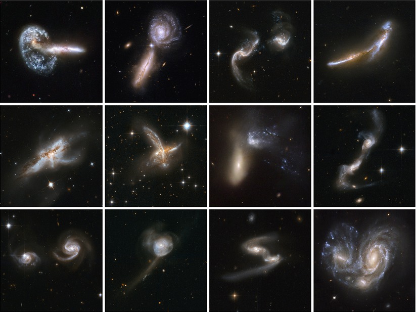
Fig. 10.1
A collection of interacting and peculiar
galaxies, as obtained by the Hubble Space Telescope. Such
interactions and mergers are partly responsible for the formation
of the current population of galaxies. Top row: Arp 148, UGC 9618, Arp 256,
NGC 6670. Middle row:
NGC 6240, ESO 593-8, NGC 454, UGC 8335. Bottom row: NGC 6786, NGC 17,
ESO 77-14, NGC 6050. Credit: NASA, ESA, the Hubble Heritage
(STScI/AURA)-ESA/Hubble Collaboration, and A. Evans (University of
Virginia, Charlottesville/NRAO/Stony Brook University)
After having described the cosmological model in
great detail, as well as the objects that inhabit our Universe at
low and high redshifts, we will now try to understand how these
objects can be formed and how they evolve in cosmic time.
The extensive results from observations of
galaxies at high redshift which were presented earlier might
suggest that the formation and evolution of galaxies is quite well
understood today. We are able to examine galaxies at redshifts up
to z ∼ 7 (and find
plausible candidates at even higher redshifts) and therefore
observe galaxies at nearly all epochs of cosmic evolution. This
seems to imply that we can study the evolution of galaxies
directly. However, this is true only to a certain degree. Although
we observe the galaxy population throughout 90 % of the cosmic
history, the relation between galaxies at different redshifts is
not easily understood. We cannot suppose that galaxies seen at
different redshifts represent various subsequent stages of
evolution of the same kind of galaxy. The main reason for this
difficulty is that different selection criteria need to be applied
to find galaxies at different redshifts.
We shall explain this point with an example.
Actively star-forming galaxies with z ≳ 2. 5 are efficiently detected by
applying the Lyman-break criterion, but only those which do not
experience much reddening by dust. Actively star-forming galaxies
at z ∼ 1 are discovered as
extremely red objects (EROs) if they are sufficiently reddened by
dust, and at z ∼ 2. 5 as
sub-millimeter galaxies. The relation between these galaxy
populations depends, of course, on how large the fraction of
galaxies is whose star-formation regions are enshrouded by dense
dust. To determine this fraction, one would need to find
Lyman-break galaxies (LBGs) at z ∼ 1, or EROs at z ∼ 3. Both observations are very
difficult today, however. For the former, this is because the Lyman
break is then located in the UV domain of the spectrum and thus can
not be observed with ground-based telescopes. For the latter it is
because the rest wavelength corresponding to the observed R-band
lies in the UV where the emission of EROs is very small, so that
virtually no optical radiation from such objects would be visible,
rendering spectroscopy of these objects impossible. In addition to
this, there is the problem that galaxies with 1. 3 ≲ z ≲ 2. 5 are difficult to discover
because, for objects at those redshifts, hardly any spectroscopic
indicators are visible in the optical range of the spectrum—both
the 4000 Å-break and the λ = 3727 Å line of [Oii] are redshifted into the NIR, as
are the Balmer lines of hydrogen, whereas the Lyman lines of
hydrogen are located in the UV part of the spectrum. For these
reasons, this range in redshift is also called the ‘redshift
desert’.1 Thus, it is
difficult to trace the individual galaxy populations as they evolve
into each other at the different redshifts. Do the LBGs at
z ∼ 3 possibly represent an
early stage of today’s ellipticals (and the passive EROs at
z ∼ 1), or are they an
early stage of spiral galaxies? Or do some galaxies form the bulk
of their stellar population at z ∼ 3, whereas others do it at some
later epoch?
The difficulties just mentioned are the reasons
why our understanding of the evolution of the galaxy population is
only possible within the framework of models, with the help of
which the different observational facts are being interpreted. We
will discuss some aspects of such models in this chapter.
Another challenge for galaxy evolution models are
the observed scaling relations of galaxy properties. We expect that
a successful theory of galaxy evolution can predict the
Tully–Fisher relation for spiral galaxies, the fundamental plane
for ellipticals, as well as the tight correlation between galaxy
properties and the central black hole mass. This latter point also
implies that the evolution of AGNs and galaxies must be considered
in parallel, since the growth of black holes with time is expected
to occur via accretion, i.e., during phases of activity in the
corresponding galaxies. The hierarchical model of structure
formation implies that high-mass galaxies form by the merging of
smaller ones (Fig. 10.1); if the aforementioned scaling relations
apply at high redshifts (and there are indications for this to be
true, although with redshift-dependent pre-factors that reflect the
evolution of the stellar population in galaxies), then the merging
process must preserve the scaling laws, at least on average.
10.1 Introduction and overview
Key
questions. In this final chapter we shall outline some of
the current ideas on the formation and evolution of galaxies, their
large-scale environment and their central black holes. We start
with a list of questions a successful model is expected to provide
answers for:
-
Why are galaxies the dominant objects in the Universe? We have seen that most of the stars live in galaxies with a luminosity which lies within a factor of ∼ 10 of the characteristic luminosity L ∗ of the Schechter function [(3.52); see also (3.59)]; what defines this characteristic luminosity (and mass) scale?
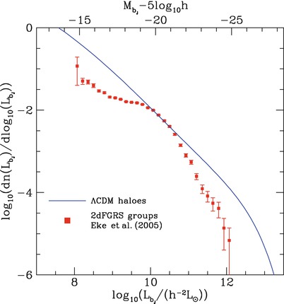 Fig. 10.2The red points with error bars show the luminosity function of galaxies and groups of galaxies as measured from the two-degree field galaxy redshift survey. In comparison, the solid curve shows the abundance of dark matter halos as predicted in a ΛCDM model, assuming a fixed mass-to-light ratio. This mass-to-light ratio is chosen such that the curves touch at one point, yielding
 . The
corresponding halo mass is M ∼ 1012 h −1 M ⊙. There is an obvious
discrepancy between the shape of the observed luminosity function
and that expected if all halos had the same mass-to-light ratio.
This implies that halos of different mass have different efficiency
with which baryons are converted into stars. In other words, the
mass-to-light ratio is smallest for halos of mass ∼ 1012
h −1
M ⊙, and the
efficiency of turning baryons into stars is suppressed for higher
and lower mass halos. Source: C.M. Baugh 2006, A primer on hierarchical galaxy formation: the
semi-analytical approach, arXiv:astro-ph/0610031, Fig. 6.
Reproduced by permission of the author
. The
corresponding halo mass is M ∼ 1012 h −1 M ⊙. There is an obvious
discrepancy between the shape of the observed luminosity function
and that expected if all halos had the same mass-to-light ratio.
This implies that halos of different mass have different efficiency
with which baryons are converted into stars. In other words, the
mass-to-light ratio is smallest for halos of mass ∼ 1012
h −1
M ⊙, and the
efficiency of turning baryons into stars is suppressed for higher
and lower mass halos. Source: C.M. Baugh 2006, A primer on hierarchical galaxy formation: the
semi-analytical approach, arXiv:astro-ph/0610031, Fig. 6.
Reproduced by permission of the author -
Can the model of structure evolution in the Universe, which is based on gravitational instability and mainly driven by dark matter inhomogeneities, explain the formation of galaxies?
-
What is the reason for the existence of two main galaxy populations, the early-types or ellipticals, and the late-type or spirals? Do they have a different evolutionary history? Can we actually understand the relative abundance of these two populations, and even their distribution in luminosity or stellar mass?
-
Why is the shape of the galaxy luminosity function different from the shape of the dark matter halo mass function (see Fig. 10.2)? In other words, what causes the different mass-to-light ratios, or stellar-to-total mass ratios, of halos?
-
The properties of the galaxy population and its relative abundance depend on the environment. Why are red galaxies the dominant population in high-density regions such as clusters, whereas blue galaxies dominate the field population?
-
Can we understand the dependence of the star-formation rate on redshift, such as is displayed in the Madau diagram (see Sect. 9.6.2)? Why has the star-formation activity declined so strongly over the past five billion years?
-
Why is the mass of the supermassive black hole in the center of galaxies so tightly linked to the stellar properties of the galaxies? Which mechanism yields the co-evolution of the mass of the central black hole and the growth of the stellar mass? Do the stellar properties determine the mass of the black hole, or reversely, does the black hole affect the evolution of the stellar population—or are both of them jointly affected by the processes of galaxy growth?
-
What is the role of active galactic nuclei in the evolution of the galaxy population? Why are some galaxies very active, some are not, and why is the fraction of active galaxies such a strong function of redshift?
-
How are the special kinds of galaxies seen at high redshift related to the local galaxy population? What is the fate of an object which we can see as sub-millimeter galaxy at z ∼ 2, or a Lyman-break galaxy at z ∼ 3—into what kind of object have they developed?
-
Why are galaxies at high redshift significantly different from local ones, in terms of size and morphology?
As we shall see, for most of these question
plausible answers can be given in the framework of the cosmological
model. The panchromatic view of cosmic sources, provided to us by a
suite of superb telescopes and instruments, allows us to link
together the evidence about the physical nature of objects obtained
from very different wavelengths. These observational results are
used to build models of the evolution of galaxies which attempt to
account for as many of them as possible. These models differ in
detail, but we currently have a rather coherent picture of the key
features that govern the formation and evolution of galaxies,
although many important issues are still to be clarified.
Overview.
The evolution of structure in the Universe is seeded by density
fluctuations which at the epoch of recombination can be observed
through the CMB anisotropy. Hence, we have direct observational
evidence about the fluctuation spectrum at z ∼ 1100. Cosmological N-body simulations predict the
evolution of the dark matter distribution as a function of
redshift, in particular the formation of halos and their merger
processes. Before recombination, baryons were coupled tightly to
the photons and thus subject to a strong pressure which prevented
them to fall into the potential wells formed by dark matter
inhomogeneities (see Sect. 7.4.3). After recombination the
baryonic matter decoupled from radiation, became essentially
pressure free, and soon followed the same spatial distribution as
the dark matter. However, baryonic matter is subject to physical
processes like dissipation, friction, heating and cooling, and star
formation. Since dark matter is not susceptible to these processes,
the behavior of baryons and the dark matter is expected to differ
in the ongoing evolution of the density field.
In the cold dark matter universe, small density
structures formed first, which means that low-mass dark matter
halos preceded those of higher mass. This ‘bottom-up’ scenario of
structure formation follows from the shape of the power spectrum of
density fluctuations, which itself is determined by the nature of
dark matter—namely cold dark matter. The gas in these halos is
compressed and heated, the source of heat being the potential
energy. If the gas is able to cool by radiative processes, i.e., to
get rid of some of its thermal energy and thus pressure, it can
collapse into denser structures, and eventually form stars. In
order for this to happen, the potential wells have to have a
minimum depth, so the resulting kinetic energy of atoms is
sufficient to excite the lowest-lying energy levels whose
de-excitation then leads to the emission of a photon which yields
the radiative cooling. We shall see that this latter aspect is
particularly relevant for the first stars to form, since they have
to be made of gas of primordial composition, i.e., only of hydrogen
and helium.
Once the first stars form in the Universe, the
baryons in their cosmic neighborhood get ionized. This reionization
at first happens locally around the most massive dark matter halos
that were formed; lateron, the individual ionized regions begin to
overlap, the remaining neutral regions become increasingly small,
until the process of reionization is completed, and the Universe
becomes largely transparent to radiation, i.e., photons can
propagate over large distances in the Universe. The gas in dark
matter halos is denser than that in intergalactic space; therefore,
the recombination rate is higher there and the gas in these halos
is more difficult to ionize. Probably, the ionizing intergalactic
radiation has a small influence on the gas in halos hosting a
massive galaxy. However, for lower-mass halos, the gas not only
maintains a higher ionization fraction, but the heating due to
ionization can be appreciable. As a result, the gas in these
low-mass halos finds it more difficult to cool and to form stars.
Thus, the star-formation efficiency—or the fraction of baryons that
is turned into stars—is expected to be smaller in low-mass
galaxies.
The mass of halos grows, either by merging
processes of smaller-mass halos or by accreting surrounding matter
through the filaments of the large-scale density field. The
behavior of the baryonic matter in these halos depends on the
interplay of various processes. If the gas in a halo can cool, it
will sink towards the center. One expects that the gas, having a
finite amount of angular momentum like the dark matter halo itself,
will initially accumulate in a disk perpendicular to the angular
momentum of the gas, as a consequence of gas friction—provided a
sufficiently long time of quiescent evolution for this to happen.
The gas in the disk then reaches densities at which efficient star
formation can set in. In this way, the formation of disk galaxies,
thus of spirals, can be understood qualitatively.
As soon as star formation sets in, it has a
feedback on the gas: the most massive stars very quickly explode as
supernovae, putting energy into the gas and thereby heating it.
This feedback then prevents that all the gas turns into stars on a
very short time-scale, providing a self-regulation mechanism of the
star-formation rate. In the accretion of additional material from
the surrounding of a dark matter halo, also additional gas is
accreted as raw material for further star formation.
When two dark matter halos with their embedded
galaxies merge, the outcome depends mainly on the mass ratio of the
halos: if one of them is much lighter than the other, its mass is
simply added to the more massive halo; the same is true for their
stars. More specific, the small-mass galaxy is disrupted by tidal
forces, in the same way as the Sagittarius dwarf galaxy is
currently destroyed in our Milky Way, with the stars being added to
the Galactic halo. If, on the other hand, the masses of the two
objects are similar, the kinematically cold disks of the two
galaxies are expected to be disrupted, the stars in both objects
obtain a large random velocity component, and the resulting object
will be kinematically hot, resembling an elliptical galaxy. In
addition, the merging of gas-rich galaxies can yield strong
compression of the gas, triggering a burst of star formation, such
as we have seen in the Antennae galaxies (see Fig. 9.25). Merging should be
particularly frequent in regions where the galaxy density is high,
in galaxy groups for instance. From the example shown in
Fig. 6.68, a large number of such merging
and collision processes are detected in galaxy clusters at high
redshift.
In parallel, the supermassive black holes in the
center of galaxies must evolve, as clearly shown by the tight
scaling relations between black hole mass and the properties of the
stellar component of galaxies (Sect. 3.8.3). The same gas that triggers
star formation, say in galaxy mergers, can be used to ‘feed’ the
central black hole. If, for example, a certain fraction of
infalling gas is accreted onto the black hole, with the rest being
transformed into stars, the parallel evolution of black hole mass
and stellar mass could be explained. In those phases where the
black hole accretes, the galaxy turns into an active galaxy; energy
from the active galactic nucleus, e.g., in the form of kinetic
energy carried by the jets, can be transmitted to the gas of the
galaxy, thereby heating it. This provides another kind of feedback
regulating the cooling of gas and star formation.
When two halos merge, both hosting a galaxy with
a central black hole, the fate of the black holes needs to be
considered. At first they will be orbiting in the resulting merged
galaxy. In this process, they will scatter off stars, transmitting
a small fraction of their kinetic energy to these stars. As a
result, the velocity of the stars on average increases and many of
them will be ‘kicked out’ of the galaxy. Through these scattering
events, the black holes lose orbital energy and sink towards the
center of the potential. Finally, they form a tight binary black
hole system which loses energy through the emission of
gravitational waves (see Sect. 7.9), until they merge. With the
planned space-based laser interferometer LISA, one expects to
detect these coalescing black hole events almost throughout the
observable Universe.
The more massive halos corresponding to groups
and clusters only form in the more recent cosmic epoch. In those
regions of space where at a later cosmic epoch a cluster will form,
the galaxy-mass halos form first—the larger-scale overdensity
corresponding to the proto-cluster promotes the formation of
galaxy-mass halos, compared to the average density region in the
Universe; this is the physical origin of galaxy bias. Therefore,
one expects the oldest massive galaxies to be located in clusters
nowadays, explaining why most massive cluster galaxies are red. In
addition, the large-scale environment provided by the cluster
affects the evolution of galaxies, e.g., through tidal stripping of
material.
In the rest of this chapter, we will elaborate on
the various processes which are essential for our understanding of
galaxy formation and evolution. In Sect. 10.2 we study the behavior
of gas in a dark matter halo, in particular consider its heating
and cooling properties; the latter obviously is most relevant for
its ability to form stars. We then turn in Sect. 10.3 to the first
generation of stars and consider their ability to reionize the
Universe; we will also briefly discuss observational evidence for
approaching the reionization epoch for the highest redshift objects
known.
The formation of disk and elliptical galaxies is
studied in Sects. 10.4 and 10.5, respectively. Here we will stress the
importance of cooling processes on the one hand, and feedback
processes that leads to gas heating on the other hand. We will also
discuss the impact of mergers on the evolution of galaxies, the
evolution of supermassive black holes, and the fate of these black
holes in the aftermath of mergers. The final two sections are
dedicated to modeling the formation and evolution of galaxies, both
in the framework of numerical simulations which include the
properties of the baryons (Sect. 10.6), and with somewhat simplified
‘semi-analytic’ models (Sect. 10.7) which, due to their great flexibility,
have guided much of our understanding of galaxy evolution over the
past two decades.
10.2 Gas in dark matter halos
We have seen in Sect. 7.5.1 how density fluctuations in
the dark matter distribution evolve into gravitationally bound and
virialized systems, the dark matter halos, through the process of
gravitationally instability. In order to understand the formation
of galaxies, we need to study the behavior of the baryons in these
dark matter halos—the baryons out of which stars form.
10.2.1 The infall of gas during halo collapse
Gas
heating. As long as the fractional overdensities are small,
the spatial distribution of baryons and dark matter are expected to
be very similar. In the language of the spherical collapse model,
initially the radial distribution of an overdense sphere is the
same for dark matter and baryons, scaled by their different mean
cosmic density. However, when the sphere collapses, the behavior of
both components must be very different: dark matter is
collisionless, and the dark matter particles can freely propagate
through the density distribution, crossing the orbits of other
particles. Baryons, on the other hand, are collisional, which means
that friction prevents gas from crossing through a gas
distribution. Thus, as the halo collapses, the potential energy of
the gas is transformed into heat through the frictional processes.
Furthermore, the pressure of the gas can prevent it from falling
into the dark matter potential well, depending on the gas
temperature and the depth of the potential well, i.e., the halo
mass. As we shall see below, this pressure effect is important for
low-mass halos at high redshifts. But first, we assume that the gas
initially is sufficiently cold such that this effect can be
neglected in the halo collapse.
In the case of (approximate) spherical symmetry,
one can picture this as follows: In the inner part of the halo, gas
has already settled down into a quasi-hydrostatic state, where gas
pressure balances the gravitational force. As the outer part of the
halo collapses, gas falls onto this gas distribution. The infall
speed is much higher than the sound velocity of the (cold)
infalling gas, i.e., the gas falls in supersonically. This is the
situation in which a shock front develops, i.e., a zone in which
gas density, pressure, and velocity varies rapidly with position
and in which the dissipation of kinetic energy (given by the infall
velocity) into heat occurs. Inside this shock front, the gas is
hot, and (almost) all of its kinetic energy gets converted into
heat.
Virial
temperature. We can now calculate the temperature of the gas
inside a halo of (total) mass M. For that, we assume that the gas
temperature T g
is uniform. According to the virial theorem, half of the potential
energy of the infalling gas is converted into kinetic energy, which
in turn is transformed into heat. We can therefore equate the
thermal energy per unit volume to one half of the potential energy
of the gas per unit volume,
 where μ m p is
the mean mass per particle in the gas, and the factor ν ∼ 1 depends on the assumed density
profile of the halo of mass M and radius r. Note that the final term in
(10.1) is just
the square of the circular velocity, V c 2. Ignoring
factors of order unity, the gas temperature will thus be similar to
the virial temperature
T vir, defined
as
where μ m p is
the mean mass per particle in the gas, and the factor ν ∼ 1 depends on the assumed density
profile of the halo of mass M and radius r. Note that the final term in
(10.1) is just
the square of the circular velocity, V c 2. Ignoring
factors of order unity, the gas temperature will thus be similar to
the virial temperature
T vir, defined
as
 Thus, a collapsed halo contains hot gas, with a temperature
depending on the halo radius and mass. Such a hot gas is seen in
galaxy groups and clusters though its X-ray emission (see
Sect. 6.4). For galaxy-mass halos, this
hot gas is much more difficult to observe: (10.2) predicts a
characteristic gas temperature for galaxy-mass halos
of ∼ 106 K. At these temperatures, gas is very difficult
to observe. The temperature is too low for being observable in
X-rays—the corresponding X-ray energies are ∼ 0. 1 keV, for which
the interstellar medium of the Milky Way is essentially opaque.
Furthermore, at these temperatures most atoms are fully ionized, so
there is little diagnostics of this gas from optical or UV line
radiation. Nevertheless, some highly (but not fully) ionized
species (such as five times ionized oxygen) exist, and their
presence can be seen through absorption lines, e.g., in the
spectrum of quasars. In this way, the presence of hot gas
surrounding our Milky Way has been established. Nevertheless, some
significant fraction the hot gas in galaxy-mass halos does not stay
hot, but must cool, otherwise stars can not form. We shall turn to
cooling processes next.
Thus, a collapsed halo contains hot gas, with a temperature
depending on the halo radius and mass. Such a hot gas is seen in
galaxy groups and clusters though its X-ray emission (see
Sect. 6.4). For galaxy-mass halos, this
hot gas is much more difficult to observe: (10.2) predicts a
characteristic gas temperature for galaxy-mass halos
of ∼ 106 K. At these temperatures, gas is very difficult
to observe. The temperature is too low for being observable in
X-rays—the corresponding X-ray energies are ∼ 0. 1 keV, for which
the interstellar medium of the Milky Way is essentially opaque.
Furthermore, at these temperatures most atoms are fully ionized, so
there is little diagnostics of this gas from optical or UV line
radiation. Nevertheless, some highly (but not fully) ionized
species (such as five times ionized oxygen) exist, and their
presence can be seen through absorption lines, e.g., in the
spectrum of quasars. In this way, the presence of hot gas
surrounding our Milky Way has been established. Nevertheless, some
significant fraction the hot gas in galaxy-mass halos does not stay
hot, but must cool, otherwise stars can not form. We shall turn to
cooling processes next.
(10.1)
(10.2)
10.2.2 Cooling of gas
In order to form stars in a halo, the gas needs
to compress to form dense clouds in which star formation occurs.
The pressure of the hot gas prevents gas from condensing further,
unless the gas can cool and thereby, at fixed pressure, increases
its density.
Cooling
processes. Optically thin gas can cool by emitting
radiation—i.e., it gets rid of some of its energy in form of
photons. There are several relevant processes by which internal
energy can be transformed into radiation. In an ionized gas, the
scattering between electrons and nuclei causes the emission of
bremsstrahlung (free-free emission), as we discussed in
Sect. 6.4.1. Collisions between atoms and
electrons can lead to a transition of an atom into an excited state
(collisional excitation). When the excited state decays
radiatively, the energy difference between the ground level and the
excited state is radiated away. Collisions can also lead to
(partial) ionization of atoms, and subsequent recombination is
again related to the emission of photons.
Cooling
function. Common to all these processes is that they depend
on the square of the gas density: they all are two-body processes
due to collisions of particles. If we define the cooling rate
C as the energy radiated
away per unit volume and unit time, then C ∝ n H 2, with
n H being the
number density of hydrogen nuclei (i.e., the sum of neutral and
ionized hydrogen atoms). The constant of proportionality is called
the cooling function,
defined as
 which depends on the gas temperature and its chemical composition.
Figure 10.3 shows the cooling function for three
different values of the gas metallicity.
which depends on the gas temperature and its chemical composition.
Figure 10.3 shows the cooling function for three
different values of the gas metallicity.
(10.3)
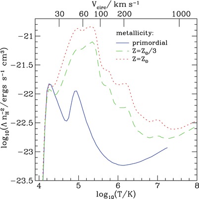
Fig. 10.3
The cooling function for gas with
primordial composition (blue solid
curve), 1/3 of the Solar metallicity (green dashed curve) and Solar
metallicity (red dotted
curve). On the top axis, the temperature is converted into a
circular velocity, according to (10.2). To obtain such a cooling function, one
needs to assume an equilibrium state of the gas. Here it is assumed
that the gas is in thermodynamical equilibrium, where the fraction
of ionization states of any atom depends just on T. The total cooling function shown
here is a superposition of different gas cooling processes,
including atomic processes and bremsstrahlung, the latter of which
dominating at high T where
the gas is fully ionized. Source: C.M. Baugh 2006, A primer on hierarchical galaxy formation: the
semi-analytical approach, arXiv:astro-ph/0610031, Fig. 9.
Reproduced by permission of the author
The relative importance and efficiency of the
various cooling processes depend on the density and temperature of
the gas, as well as on its chemical composition. At very high
temperatures, all atoms are fully ionized, and thus the processes
of collisional excitation and ionization are no longer of
relevance. Then, bremsstrahlung becomes the dominant effect, with
Λ(T) ∝ T 1∕2 [see also
(6.32)]. This behavior is seen in
Fig. 10.3 for
a pure hydrogen plus helium gas at T ≳ 106 K; for gas with
non-zero metallicity, bremsstrahlung starts to dominate the cooling
at somewhat higher temperatures.
For gas with primordial abundance, we see two
clear peaks in the cooling function in Fig. 10.3, one at T ∼ 2 × 10⁴ K, the other at
T ∼ 105 K. The
former one is due to the fact that for gas at this temperature,
hydrogen is mostly neutral, and many particles in the gas have an
energy sufficient for the excitation of higher energy levels in
hydrogen atoms; note that the lowest lying excited state of
hydrogen has an energy corresponding to the Lyman-α transition, i.e., 10. 2 eV,
corresponding to a temperature of T ∼ 105 K. Thus, collisional
excitation is efficient. At slightly higher temperatures, also
collisional ionization (and subsequent recombination) is very
effective, but with increasing T, the cooling function drops, because
then hydrogen becomes mostly ionized. The second peak has the same
origin, except that now the helium atom is the main coolant. Since
the lowest energy level and the ionization energy in helium is
higher than for hydrogen, the helium peak is simply shifted. Once
helium is fully ionized, atomic cooling shuts off, and only at
higher temperatures the bremsstrahlung effect takes over.
Although elements heavier than helium have a
small abundance in number, they can dominate the gas cooling, due
to the rich energy spectrum of many-electron atoms. The cooling
function for gas with Solar metallicity is larger by more than an
order of magnitude than that of primordial gas, over a broad range
of temperatures. Hence, more enriched gas finds it easier to
cool.
Atomic gas cannot cool efficiently for
temperatures T ≲ 104 K, due to the lack
of charged particles (electrons and ions) in the gas. However, in
chemically enriched gas, the few free electrons present at
T ≲ 104 K can
excite low-energy states (the so-called fine-structure levels) of
ions like that of oxygen or carbon. Molecules, on the other hand,
have a rich spectrum of energy levels at considerably smaller
energies, and can therefore lead to efficient cooling towards lower
temperatures. This is the reason why star formation occurs in
molecular clouds, where gas can efficiently cool and thereby
compress to high densities.
Cooling
time. Once we know the rate at which gas loses its energy,
we can calculate the cooling time, the time it takes the gas (at
constant cooling rate) to lose all of its energy:
 If this cooling time is longer than the age of the Universe, then
the gas essentially stays at the same temperature and is unable to
collapse towards the halo center. We have seen in
Sect. 6.4.3 that for most regions in
clusters, this is indeed the case; only in the central regions of
clusters cooling can be effective.
If this cooling time is longer than the age of the Universe, then
the gas essentially stays at the same temperature and is unable to
collapse towards the halo center. We have seen in
Sect. 6.4.3 that for most regions in
clusters, this is indeed the case; only in the central regions of
clusters cooling can be effective.
(10.4)
Free-fall
time. On the other hand, if the cooling time is sufficiently
short, gas can compress towards the halo center. What ‘sufficiently
short’ means can be seen if we compare the cooling time with the
free-fall time, i.e., the time it takes a freely falling particle
at some radius r in the
halo to reach the center. The free-fall time depends only on the
mean total mass density (i.e., dark matter plus baryons) inside
r (see problem 4.7)
and is given by
 where we used the gas-mass fraction
  to convert
the total density to the gas density, which was then expressed in
terms of the particle number density n by ρ g = n μ m p.
to convert
the total density to the gas density, which was then expressed in
terms of the particle number density n by ρ g = n μ m p.
(10.5)
to convert
the total density to the gas density, which was then expressed in
terms of the particle number density n by ρ g = n μ m p.Conditions for
efficient cooling. If the cooling time is shorter than the
free-fall time, then gas falls freely towards the center,
essentially unaffected by gas pressure. If, on the other hand, the
cooling time is much longer than the free-fall time, the gas at
best sinks to the center at a rate given by the cooling rate—this
is similar to the cooling flows discussed in Sect. 6.4.3. Hence, in this case, cooling
is rather inefficient.
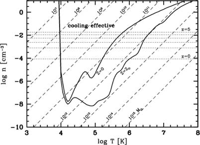
Fig. 10.4
The solid
curves in this cooling diagram show the density as a
function of temperature, for which t cool = t ff, both for gas with
primordial abundance (Z = 0) and with Solar abundance
(Z = Z ⊙). Note that this
condition yields ![$$n \propto f_{\mathrm{g}}^{-1}\left [T/\varLambda (T)\right ]^{2}$$](A129044_2_En_10_Chapter_IEq3.gif) ,
and so these curves are similar to the inverse of the cooling
function in Fig. 10.3. Here, the gas fraction was chosen to
correspond to its cosmic mean f g = 0. 15. Dotted horizontal lines indicate the
density of halos which form at the indicated redshifts, which is
determined by the fact that the mean density of a halo is ∼ 200
times the critical density of the Universe at this epoch. The
diagonal dashed lines show
the n-T relation for fixed gas mass
M g, which is
obtained from (10.2), r ∝ M∕T and the fact that M g ∝ r 3 n. Eliminating r from these two relations yields
,
and so these curves are similar to the inverse of the cooling
function in Fig. 10.3. Here, the gas fraction was chosen to
correspond to its cosmic mean f g = 0. 15. Dotted horizontal lines indicate the
density of halos which form at the indicated redshifts, which is
determined by the fact that the mean density of a halo is ∼ 200
times the critical density of the Universe at this epoch. The
diagonal dashed lines show
the n-T relation for fixed gas mass
M g, which is
obtained from (10.2), r ∝ M∕T and the fact that M g ∝ r 3 n. Eliminating r from these two relations yields
 .
Source: H. Mo, F. van den Bosch & S. White 2010, Galaxy Formation and Evolution,
Cambridge University Press, p. 386. Reproduced by permission of the
author
.
Source: H. Mo, F. van den Bosch & S. White 2010, Galaxy Formation and Evolution,
Cambridge University Press, p. 386. Reproduced by permission of the
author
,
and so these curves are similar to the inverse of the cooling
function in Fig. 10.3. Here, the gas fraction was chosen to
correspond to its cosmic mean f g = 0. 15. Dotted horizontal lines indicate the
density of halos which form at the indicated redshifts, which is
determined by the fact that the mean density of a halo is ∼ 200
times the critical density of the Universe at this epoch. The
diagonal dashed lines show
the n-T relation for fixed gas mass
M g, which is
obtained from (10.2), r ∝ M∕T and the fact that M g ∝ r 3 n. Eliminating r from these two relations yields
.
Source: H. Mo, F. van den Bosch & S. White 2010, Galaxy Formation and Evolution,
Cambridge University Press, p. 386. Reproduced by permission of the
authorThus, the condition t cool = t ff separates situations in
which gas can easily fall inside the halo and form denser gas
concentrations from those where gas compression is prevented. In
Fig. 10.4,
this condition is shown as solid curves, both for primordial gas
and gas with Solar abundance. For gas densities and temperature
above the curves, cooling is efficient, whereas the cooling time is
longer than the free-fall time below the curves.
The dotted horizontal lines in Fig. 10.4 indicate the mean gas
density of halos collapsed at the redshift indicated, assuming a
halos gas-mass fraction of f g = 0. 15, i.e., about the
cosmic average (recall that a halo has about 200 times the critical
density of the Universe at the epoch of halo formation). Thus, for
the cooling of gas in halos, only the region above the dotted lines
is relevant. For each redshift, there is a range in temperatures
for which gas can cool efficiently.
Finally, the dashed diagonal lines indicate the
density n as a function of
temperature, for a fixed mass M g as indicated. For
 , the
dashed line lies below the solid curves for all T; hence, gas in halos with mass
, the
dashed line lies below the solid curves for all T; hence, gas in halos with mass
 cannot
cool. Even for
cannot
cool. Even for  , the dashed
curve lies mostly outside the region where cooling is efficient,
even for Solar abundance, except below the dotted lines, i.e., at
densities which are smaller than the mean densities of halos. But
if gas cannot cool, gas condensation and star formation is
inefficient.
, the dashed
curve lies mostly outside the region where cooling is efficient,
even for Solar abundance, except below the dotted lines, i.e., at
densities which are smaller than the mean densities of halos. But
if gas cannot cool, gas condensation and star formation is
inefficient.
, the
dashed line lies below the solid curves for all T; hence, gas in halos with mass
cannot
cool. Even for , the dashed
curve lies mostly outside the region where cooling is efficient,
even for Solar abundance, except below the dotted lines, i.e., at
densities which are smaller than the mean densities of halos. But
if gas cannot cool, gas condensation and star formation is
inefficient.The difference
between galaxies and groups/clusters. From Fig. 10.4, we can thus draw a
first important conclusion: In sufficiently massive halos with
 , the small
efficiency of gas cooling prevents gas from collapsing to the
center and forming stars there. At smaller masses, cooling is
effective to enable rapid gas collapse. This dividing line in mass
is about the mass which distinguishes galaxies from groups and
clusters. In the latter, only a small fraction of the baryons is
turned into stars, and these are contained in the galaxies within
the group; the group halo itself does not contain stars, with the
exception of the intracluster light. But as we discussed in
Sect. 6.3.4, these stars most likely have
been stripped from galaxies in groups through interactions. In
contrast, a large fraction of baryons in galaxies is concentrated
towards the center, as visible in their stellar distribution. Thus,
the difference between galaxies and groups/clusters is their
efficiency to turn baryons into stars, and this difference is
explained with the different cooling efficiency shown in
Fig. 10.4.
, the small
efficiency of gas cooling prevents gas from collapsing to the
center and forming stars there. At smaller masses, cooling is
effective to enable rapid gas collapse. This dividing line in mass
is about the mass which distinguishes galaxies from groups and
clusters. In the latter, only a small fraction of the baryons is
turned into stars, and these are contained in the galaxies within
the group; the group halo itself does not contain stars, with the
exception of the intracluster light. But as we discussed in
Sect. 6.3.4, these stars most likely have
been stripped from galaxies in groups through interactions. In
contrast, a large fraction of baryons in galaxies is concentrated
towards the center, as visible in their stellar distribution. Thus,
the difference between galaxies and groups/clusters is their
efficiency to turn baryons into stars, and this difference is
explained with the different cooling efficiency shown in
Fig. 10.4.This effect partly answers one of the questions
posed at the start of this chapter. The mass-to-light ratio of very
massive halos is much larger than that of galaxies (see
Fig. 10.2)
because of the much longer cooling time of the gas. In groups and
clusters, most of the gas is present in the form of a hot gaseous
halo.
Low-mass
halos. Another conclusion we might want to draw from this
cooling diagram is the behavior of halos at the low-mass end. A
halo with gas mass  lies inside the cooling
curve only at very high
redshift, i.e., when the corresponding density in a halo is very
high. Therefore, gas can cool, and stars form, in halos of this
mass only if they formed early enough. We therefore expect that the
stars in such low-mass halos are very old. We will soon find that
there are additional effects which further strengthen this
conclusion. Combined, these effects provide a natural explanation
for the ‘missing satellite’ problem discussed in Sect. 7.8.
lies inside the cooling
curve only at very high
redshift, i.e., when the corresponding density in a halo is very
high. Therefore, gas can cool, and stars form, in halos of this
mass only if they formed early enough. We therefore expect that the
stars in such low-mass halos are very old. We will soon find that
there are additional effects which further strengthen this
conclusion. Combined, these effects provide a natural explanation
for the ‘missing satellite’ problem discussed in Sect. 7.8.Cold accretion vs.
hot accretion. The cooling diagram in Fig. 10.4 is very useful to
discuss such properties qualitatively. Of course, the assumptions
made to derive it are quite simple and idealized, such as the
consideration of just the mean gas density, instead of a density
profile, and the neglect of further effects, such as merging of
halos.
A more realistic consideration needs to account
for the fact that the gas is not homogeneous. The quasi-hydrostatic
density profile implies that the gas density increases towards the
center. In the inner part, it may be dense enough for cooling to be
effective. In such halos, we therefore expect to have a central
concentration of cold gas, surrounded by a hot gaseous halo with a
temperature close to the virial temperature.
Furthermore, the implicit assumption of spherical
symmetry made above may be misleading. From simulations of
structure formation (see Sect. 7.5.3) we have seen that dark
matter halos are embedded in a network of sheets and filaments,
with massive halos forming at the intersection of filaments. Once
formed, such halos accrete further matter, both dark and baryonic
matter. In case of spherical symmetry, the gas would fall in and be
heated through an accretion shock, as described before. However,
the infall of matter occurs predominantly along the directions of
the filaments connected to the halo, forming streams of gas which
can reach the central regions of the halo without being strongly
heated. Hydrodynamic simulations have identified this mode of
accretion as an important route for halos to attain or replenish
their gas.
10.3 Reionization of the Universe
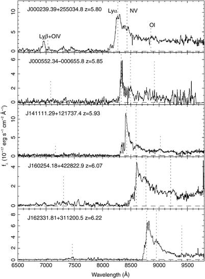
Fig. 10.5
Spectra of five QSOs at redshifts
z > 5. 7, discovered in
multi-color data from the Sloan Digital Sky Survey. The positions
of the most important emission lines are marked. Particularly
remarkable is the almost complete lack of flux bluewards of the
Lyα emission line in some
of the QSOs, indicating a strong Gunn–Peterson effect. However,
this absorption is not complete in all QSOs, which points at strong
variations in the density of neutral hydrogen in the intergalactic
medium at these high redshifts. Either the hydrogen density varies
strongly for different lines-of-sight, or the degree of ionization
is very inhomogeneous. Source: X. Fan et al. 2004,
A Survey of z > 5.7 Quasars in
the Sloan Digital Sky Survey. III. Discovery of Five Additional
Quasars, AJ 128, 515, p. 517, Fig. 1. ©AAS. Reproduced with
permission
After recombination at z ∼ 1100, the intergalactic gas became
neutral, with a residual ionization fraction of
only ∼ 10−4. Had the Universe remained neutral we would
not be able to receive any photons that were emitted bluewards of
the Lyα line of a source,
because the absorption cross section for Lyα photons is too large [see
(8.27)]. Since such photons are
observed from QSOs, as can be seen for instance in the spectra of
the z > 5. 7 QSOs in
Fig. 10.5, and
since an appreciable fraction of homogeneously distributed neutral
gas in the intergalactic medium can be excluded for z ≲ 5, from the tight upper bounds on
the strength of the Gunn–Peterson effect (Sect. 8.5.1), the Universe must have been
reionized between the recombination epoch and the redshift
z ∼ 7 of the most distant
known QSOs. As we have seen in Sect. 8.6.6, the anisotropies of the CMB
led us to conclude that reionization occurred at z ∼ 10.
This raises the question of how this reionization
proceeded, in particular which process was responsible for it. The
latter question is easy to answer—reionization must have happened
by photoionization. Collisional ionization can be ruled out because
for it to be efficient the intergalactic medium (IGM) would need to
be very hot, a scenario which can be excluded due to the perfect
Planck spectrum of the CMB—the argument here is the same as in
Sect. 9.5.3, where we excluded the idea
of a hot IGM as the source of the cosmic X-ray background. Hence,
the next question is what produced the energetic photons that
caused the photoionization of the IGM.
Two kinds of sources may in principle account for
them—hot stars or AGNs. Currently, it is not unambiguously clear
which of these is the predominant source of energetic photons
causing reionization since our current understanding of the
formation of supermassive black holes is still insufficient.
However, it is currently thought that the main source of
photoionization photons is the first generation of hot stars.
10.3.1 The first stars
Following on from the above arguments,
understanding reionization is thus directly linked to studying the
first generation of stars. In the present Universe star formation
occurs in galaxies; thus, one needs to examine when the first
galaxies could have formed. From the theory of structure formation,
the mass spectrum of dark matter halos at a given redshift can be
computed by means of, e.g., the Press–Schechter model (see
Sect. 7.5.2). Two conditions need to be
fulfilled for stars to form in these halos. First, gas needs to be
able to fall into the dark halos. Since the gas has a finite
temperature, pressure forces may impede the infall into the
potential well. Second, this gas also needs to be able to cool,
condensing into clouds in which stars can then be formed, a process
that we considered in the preceding section.
The Jeans
mass. By means of a simple argument, we can estimate under
which conditions pressure forces are unable to prevent the infall
of gas into a potential well. To do this, we consider a slightly
overdense spherical region of radius R whose density is only a little larger
than the mean cosmic matter density  . If this sphere is homogeneously filled
with baryons, the gravitational binding energy of the gas is about
. If this sphere is homogeneously filled
with baryons, the gravitational binding energy of the gas is about
 where M and M g denote the total mass
and the gas mass of the sphere, respectively. The thermal energy of
the gas can be computed from the kinetic energy per particle,
multiplied by the number of particles in the gas, or
where M and M g denote the total mass
and the gas mass of the sphere, respectively. The thermal energy of
the gas can be computed from the kinetic energy per particle,
multiplied by the number of particles in the gas, or
 is the speed of sound in the gas, which is about the average
velocity of the gas particles, and μ m p denotes, as before,
the average particle mass in the gas. For the gas to be bound in
the gravitational field, its gravitational binding energy needs to
be larger than its thermal energy, | E grav | > E th, which yields the
condition GM > c s 2
R. Since we have assumed an
only slightly overdense region, the relation
is the speed of sound in the gas, which is about the average
velocity of the gas particles, and μ m p denotes, as before,
the average particle mass in the gas. For the gas to be bound in
the gravitational field, its gravitational binding energy needs to
be larger than its thermal energy, | E grav | > E th, which yields the
condition GM > c s 2
R. Since we have assumed an
only slightly overdense region, the relation  between mass and radius
of the sphere applies. From the two latter equations, the radius
can be eliminated, yielding the condition
between mass and radius
of the sphere applies. From the two latter equations, the radius
can be eliminated, yielding the condition

. If this sphere is homogeneously filled
with baryons, the gravitational binding energy of the gas is about
between mass and radius
of the sphere applies. From the two latter equations, the radius
can be eliminated, yielding the condition
(10.6)
where the numerical coefficient is obtained from
a more accurate treatment. Thus, as a result of our simple argument
we find that the mass of the halo needs to exceed a certain
threshold for gas to be able to fall in. The expression on the
right-hand side of (10.6) defines the Jeans mass M J, which
describes the minimum mass of a halo required for the gravitational
infall of gas. The Jeans mass depends on the temperature of the
gas, expressed through the sound speed c s, and on the mean cosmic
matter density  . The latter can easily be expressed as
a function of redshift,
. The latter can easily be expressed as
a function of redshift,  .
.
. The latter can easily be expressed as
a function of redshift, .The baryon temperature T b has a more complicated
dependence on redshift. For sufficiently high redshifts, the small
fraction of free electrons that remains after recombination
provides a thermal coupling of the baryons to the cosmic background
radiation, by means of Compton scattering. This is the case for
redshifts z ≳ z t, where

hence,  for
z ≳ z t. For smaller redshifts,
the density of photons gets too small to maintain this coupling,
and baryons start to adiabatically cool down by the expansion, so
that for z ≲ z t we obtain approximately
for
z ≳ z t. For smaller redshifts,
the density of photons gets too small to maintain this coupling,
and baryons start to adiabatically cool down by the expansion, so
that for z ≲ z t we obtain approximately
 (see problem 4.9).
for
z ≳ z t. For smaller redshifts,
the density of photons gets too small to maintain this coupling,
and baryons start to adiabatically cool down by the expansion, so
that for z ≲ z t we obtain approximately
(see problem 4.9).From these temperature dependences, the Jeans
mass can then be calculated as a function of redshift. For
 ,
M J is
independent of z because
,
M J is
independent of z because
 and
and  , and its value is

,
M J is
independent of z because
and , and its value is
(10.7)
whereas for  we obtain, with
 ,
,
 Hence, gas can not fall into halos with mass lower than these
values.
Hence, gas can not fall into halos with mass lower than these
values.
we obtain, with
,
(10.8)
Cooling of the
gas. The Jeans criterion is a necessary condition for the
formation of proto-galaxies, i.e., dark matter halos which contain
baryons. In order to form stars, the gas in the halos needs to be
able to cool further. Here, we are dealing with the particular
situation of the first galaxies, whose gas is metal-free, so metal
lines cannot contribute to the cooling. As we have seen in
Fig. 10.3, the
cooling function of primordial gas is much smaller than that of
enriched material; in particular, the absence of metals means that
even slow cooling though excitation of fine-structure lines cannot
occur, as there are no atoms with such transitions present. Thus,
cooling by the primordial gas is efficient only above  . However, the
halos formed at high redshift have low mass. We have seen in
Sect. 7.5.2 that the abundance of dark
matter halos depends on the parameter ν in (7.51),
given by the product of the density fluctuations on a given mass
scale and the growth factor. At high redshift, the growth factor
D +(a) is small, and thus to have a
noticeable abundance of halos of mass M, σ(M) must be correspondingly large. At
redshift z ∼ 10, the
parameter ν is about unity
for halos of mass
. However, the
halos formed at high redshift have low mass. We have seen in
Sect. 7.5.2 that the abundance of dark
matter halos depends on the parameter ν in (7.51),
given by the product of the density fluctuations on a given mass
scale and the growth factor. At high redshift, the growth factor
D +(a) is small, and thus to have a
noticeable abundance of halos of mass M, σ(M) must be correspondingly large. At
redshift z ∼ 10, the
parameter ν is about unity
for halos of mass  . Hence, at that time,
substantially more massive halos than that were (exponentially)
rare—i.e., only low-mass halos were around, and their virial
temperature
. Hence, at that time,
substantially more massive halos than that were (exponentially)
rare—i.e., only low-mass halos were around, and their virial
temperature
 is considerably below the energy scale where atomic hydrogen can
efficiently cool. To derive (10.9), we have replaced V c in (10.2) in favor of halo
mass and radius, and used the fact that the mean matter density of
a halo inside its virial radius is ∼ 200 times the critical density
at a given redshift. Therefore, atomic hydrogen is a very
inefficient coolant for these first halos, insufficient to initiate
the formation of stars. Furthermore, helium is of no help in this
context, since its excitation temperature is even higher than that
of hydrogen.
is considerably below the energy scale where atomic hydrogen can
efficiently cool. To derive (10.9), we have replaced V c in (10.2) in favor of halo
mass and radius, and used the fact that the mean matter density of
a halo inside its virial radius is ∼ 200 times the critical density
at a given redshift. Therefore, atomic hydrogen is a very
inefficient coolant for these first halos, insufficient to initiate
the formation of stars. Furthermore, helium is of no help in this
context, since its excitation temperature is even higher than that
of hydrogen.
. However, the
halos formed at high redshift have low mass. We have seen in
Sect. 7.5.2 that the abundance of dark
matter halos depends on the parameter ν in (7.51),
given by the product of the density fluctuations on a given mass
scale and the growth factor. At high redshift, the growth factor
D +(a) is small, and thus to have a
noticeable abundance of halos of mass M, σ(M) must be correspondingly large. At
redshift z ∼ 10, the
parameter ν is about unity
for halos of mass . Hence, at that time,
substantially more massive halos than that were (exponentially)
rare—i.e., only low-mass halos were around, and their virial
temperature
(10.9)
The importance of
molecular hydrogen. Besides atomic hydrogen and helium, the
primordial gas contains a small fraction of molecular hydrogen
which represents an extremely important component in cooling
processes. Whereas in enriched gas, molecular hydrogen is formed on
dust particles, the primordial gas had no dust, and so
H2 must form in the gas phase itself, rendering its
abundance very small. However, despite its very small density and
transition probability, H2 dominates the cooling rate of
primordial gas at temperatures below T ∼ 104 K—see
Fig. 10.6—where the precise value of this temperature
depends on the abundance of H2.
By means of H2, the gas can cool in
halos with a temperature exceeding about  ,
corresponding to a halo mass of
,
corresponding to a halo mass of  at z ∼ 20. In these halos, stars may then
be able to form. These stars will certainly be different from those
known to us, because they do not contain any metals. Therefore, the
opacity of the stellar plasma is much lower. Such stars, which at
the same mass presumably have a much higher temperature and
luminosity (and thus a shorter lifetime), are called population III stars. Due to their high
temperature they are much more efficient sources of ionizing
photons than stars with ‘normal’ metallicity.
at z ∼ 20. In these halos, stars may then
be able to form. These stars will certainly be different from those
known to us, because they do not contain any metals. Therefore, the
opacity of the stellar plasma is much lower. Such stars, which at
the same mass presumably have a much higher temperature and
luminosity (and thus a shorter lifetime), are called population III stars. Due to their high
temperature they are much more efficient sources of ionizing
photons than stars with ‘normal’ metallicity.
,
corresponding to a halo mass of at z ∼ 20. In these halos, stars may then
be able to form. These stars will certainly be different from those
known to us, because they do not contain any metals. Therefore, the
opacity of the stellar plasma is much lower. Such stars, which at
the same mass presumably have a much higher temperature and
luminosity (and thus a shorter lifetime), are called population III stars. Due to their high
temperature they are much more efficient sources of ionizing
photons than stars with ‘normal’ metallicity.10.3.2 The reionization process
Dissociation of
molecular hydrogen. The energetic photons from these
population III stars are now capable of ionizing hydrogen in their
vicinity. More important still is another effect: photons with
energy above 11.26 eV can destroy H2. Since the Universe
is transparent for photons with energies below 13.6 eV, photons
with  can propagate very long distances and dissociate molecular
hydrogen. This means that as soon as the first stars have formed in
a region of the Universe, molecular hydrogen in their vicinities
will be destroyed and further gas cooling and star formation will
then be prevented.2
At this point, the Universe contains a low number density of
isolated bubbles of ionized hydrogen, centered on those halos in
which population III stars were able to form early, but this
constitutes only a tiny fraction of the volume; most of the baryons
remain neutral.
can propagate very long distances and dissociate molecular
hydrogen. This means that as soon as the first stars have formed in
a region of the Universe, molecular hydrogen in their vicinities
will be destroyed and further gas cooling and star formation will
then be prevented.2
At this point, the Universe contains a low number density of
isolated bubbles of ionized hydrogen, centered on those halos in
which population III stars were able to form early, but this
constitutes only a tiny fraction of the volume; most of the baryons
remain neutral.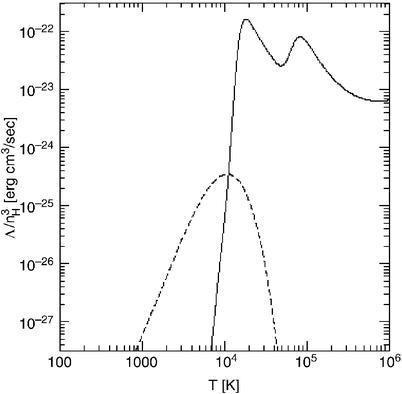
Fig. 10.6
Cooling rate as a function of the
temperature for a gas consisting of atomic and molecular hydrogen
(with 0.1 % abundance) and of helium. The solid curve describes the cooling by
atomic gas, the dashed
curve that by molecular hydrogen; thus, the latter is
extremely important at temperatures below ∼ 104 K. At
considerably lower temperatures the gas cannot cool, hence no star
formation can take place. Source: R. Barkana & A. Loeb 2000,
In the Beginning: The First
Sources of Light and the Reionization of the Universe,
astro-ph/0010468, Fig. 12. Reproduced by permission of the
author
Metal enrichment
of the intergalactic medium. Soon after population III stars
have formed, they will explode as supernovae. Through this process,
the metals produced by them are ejected into the intergalactic
medium, by which the initial metal enrichment of the IGM occurs.
The kinetic energy transferred by SNe to the gas within the halo
can exceed its binding energy, so that the baryons of the halo can
be blown away and further star formation is prevented. Whether this
effect may indeed lead to gas-free halos, or whether the released
energy can instead be radiated away, depends on the geometry of the
star-formation regions. In any case, it can be assumed that in
those halos where the first generation of stars was born, further
star formation was considerably suppressed, particularly since all
molecular hydrogen was destroyed.
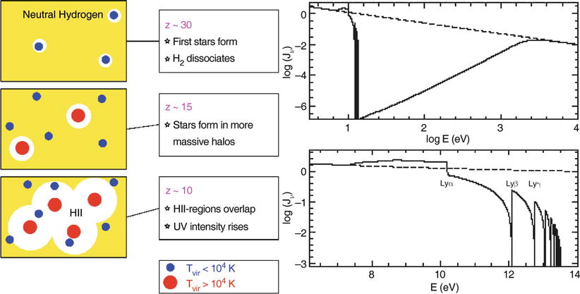
Fig. 10.7
On the
left, a sketch of the geometry of reionization is shown:
initially, relatively low-mass halos collapse, a first generation
of stars ionizes and heats the gas in and around these halos. By
heating, the temperature increases so strongly (to about
T ∼ 104 K) that
gas can escape from the potential wells; these halos may never
again form stars efficiently. Only when more massive halos have
collapsed will continuous star formation set in. Ionizing photons
from this first generation of hot stars produce Hii-regions around their halos, which
is the onset of reionization. The regions in which hydrogen is
ionized will grow until they start to overlap; at that time, the
flux of ionizing photons will strongly increase. On the right, the average spectrum of
photons at the beginning of the reionization epoch is shown; here,
it has been assumed that the flux from the radiation source follows
a power law (dashed curve).
Photons with an energy higher than that of the Lyα transition are strongly suppressed
because they are efficiently absorbed. The spectrum near the Lyman
limit shows features which are produced by the combination of
breaks corresponding to the various Lyman lines, and the
redshifting of the photons. Source: R. Barkana & A. Loeb 2000,
In the Beginning: The First
Sources of Light and the Reionization of the Universe,
astro-ph/0010468, Figs. 4, 11. Reproduced by permission of the
author
We can assume that the metals produced in these
first SN explosions are, at least partially, ejected from the halos
into the intergalactic medium, thus enriching the latter. The
existence of metal formation in the very early Universe is
concluded from the fact that even sources at very high redshift
(like QSOs at z ∼ 6) have a
metallicity of about one tenth the Solar value. Furthermore, the
Lyα forest also contains
gas with non-vanishing metallicity. Since the Lyα forest is produced by the
intergalactic medium, this therefore must have been enriched.
The final step to
reionization. For gas to cool in halos without molecular
hydrogen, their virial temperature needs to exceed about
104 K (see Fig. 10.6). Halos of this virial temperature form
with appreciable abundance at redshifts of z ∼ 10, corresponding to a halo mass of
 , as can be estimated from the
Press–Schechter model (see Sect. 7.5.2). In these halos, efficient
star formation can then take place and the first proto-galaxies
form. These then ionize the surrounding IGM in the form of
Hii-regions, as sketched
in Fig. 10.7.
The corresponding Hii-regions expand because
increasingly more photons are produced. If the halo density is
sufficiently high, these Hii-regions start to overlap and soon
after, to fill the whole volume. Once this occurs, the IGM is
ionized, and reionization is completed.
, as can be estimated from the
Press–Schechter model (see Sect. 7.5.2). In these halos, efficient
star formation can then take place and the first proto-galaxies
form. These then ionize the surrounding IGM in the form of
Hii-regions, as sketched
in Fig. 10.7.
The corresponding Hii-regions expand because
increasingly more photons are produced. If the halo density is
sufficiently high, these Hii-regions start to overlap and soon
after, to fill the whole volume. Once this occurs, the IGM is
ionized, and reionization is completed.We therefore conclude that reionization is a
two-stage process. In a first phase, population III stars form
through cooling of gas by molecular hydrogen, which is then
destroyed by these very stars. Only in a later epoch and in more
massive halos cooling is provided by atomic hydrogen, leading to
reionization.
Escape fraction of
ionizing photons. We note that only a small fraction of the
baryons needs to undergo nuclear fusion in hot stars to ionize all
hydrogen, as we can easily estimate: by fusing four H-nuclei
(protons) to He, an energy of about 7 MeV per nucleon is released.
However, only 13.6 eV per hydrogen atom is required for ionization.
Hence, from a purely energetic point of view, reionization is not
particularly demanding.
The number density of hot stars required to
reionize the Universe is uncertain due to the unknown escape
fraction f esc
of ionizing photons from the first galaxies, i.e., the ratio of the
number of ionizing photons which can propagate out of the galaxy to
the total number of ionizing photons produced by hot stars. Photons
with energy E
γ ≥ 13. 6 eV
are easily absorbed by the neutral fraction of the gas. For local
star-forming galaxies, the escape fraction can be estimated to be
between a few percent up to ∼ 0. 5. However, the first galaxies
that formed were denser. Furthermore, the escape fraction depends
on the geometrical arrangement of the hot stars relative to the
interstellar medium, as well as the clumpiness of the latter. If
the stars are located in the inner part of the galaxy, surrounded
by a smooth interstellar medium, the escape fraction will be very
small. If, however, the ISM is clumpy such that it only occupies a
small fraction of the volume, photons can escape ‘between the
clumps’, and the escape fraction can be appreciable. There is also
the possibility that the star formation and subsequent supernovae
drive much of the gas out of the galaxy halos, increasing the
escape fraction for later stellar generations.
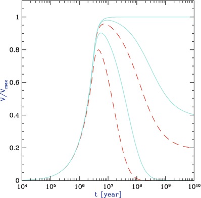
Fig. 10.8
The volume of an expanding Hii region from an instantaneous
starburst, normalized to the maximally possible volume V max (which is given by
equating the number of hydrogen atoms  with the total number of ionizing photons generated by the
starburst). The upper solid
curve assumes that no recombination takes place. The two
other solid curves assume
that the starburst occurs at redshift z = 10, and that the intergalactic
medium is uniform (middle solid
curve) or strongly clumped (lower solid curve). The two
dashed curves show the
same, except that for them, z = 15 is assumed; since the density is
higher at larger redshift, the recombination rate is accordingly
higher. Source: R. Barkana & A. Loeb 2000, In the Beginning: The First Sources of Light
and the Reionization of the Universe, astro-ph/0010468,
Fig. 21. Reproduced by permission of the author
with the total number of ionizing photons generated by the
starburst). The upper solid
curve assumes that no recombination takes place. The two
other solid curves assume
that the starburst occurs at redshift z = 10, and that the intergalactic
medium is uniform (middle solid
curve) or strongly clumped (lower solid curve). The two
dashed curves show the
same, except that for them, z = 15 is assumed; since the density is
higher at larger redshift, the recombination rate is accordingly
higher. Source: R. Barkana & A. Loeb 2000, In the Beginning: The First Sources of Light
and the Reionization of the Universe, astro-ph/0010468,
Fig. 21. Reproduced by permission of the authorClumpiness of the
intergalactic medium. A further uncertainty in the
quantitative understanding of reionization lies in the clumpiness
of the intergalactic medium. An ionized hydrogen atom may become
neutral again due to recombination. Hence, one may need more than
one ionizing photon per atom for complete reionization. Since
recombination is a two-body process (i.e., its rate depends
quadratically on the gas density), its relative importance depends
on the redshift of reionization and the clumpiness of the gas
distribution: The higher the redshift, the larger the density of
the intergalactic medium, and the higher the recombination rate.
Clumpiness also increases the mean of the squared gas density,
yielding a higher mean recombination rate (see Fig. 10.8).
Once reionization is completed, the intergalactic
medium has a temperature of about 104 K, due to the
heating of the gas by photoionization: the typical energy of a
photon which ionizes a hydrogen atom is somewhat larger than
13. 6 eV, and the energy difference is transferred to the electron,
which is tightly coupled by Coulomb interactions with the other gas
particles. Thus, this surplus energy causes a heating of the gas.
The resulting temperature depends on the spectrum of the ionizing
radiation; the harder the spectrum, the higher the
temperature.
Suppression of
low-mass galaxies. The increase of temperature causes an
increase of the Jeans mass (10.6), due to its dependence on the sound
velocity. Once the intergalactic medium is heated
to ∼ 104 K by intergalactic UV radiation, the gas
pressure prevents gas inflow into low-mass halos,
corresponding3 to
circular velocities ≲ 30 km∕s. For this reason, one expects that
halos of lower mass have a lower baryon fraction than that of the
cosmic mixture,  .
The actual value of the baryon fraction depends on the details of
the merger history of a halo. Quantitative studies yield an average
baryon mass of
.
The actual value of the baryon fraction depends on the details of
the merger history of a halo. Quantitative studies yield an average
baryon mass of
![$$\displaystyle{ \bar{M}_{\mathrm{b}} = \frac{f_{\mathrm{b}}\,M} {\left [1 + (2^{\alpha /3} - 1)(M_{\mathrm{C}}/M)^{\alpha }\right ]^{(3/\alpha )}}\;, }$$](A129044_2_En_10_Chapter_Equ10.gif) where
where  is a
characteristic mass, defined such that for a halo with mass
M C,
is a
characteristic mass, defined such that for a halo with mass
M C,
 . For
halos of mass smaller than M C, the baryon fraction is
suppressed, decreasing as (M∕M C)3 for small
masses, whereas for halo masses ≫ M C, the baryon fraction
corresponds to the cosmic average. The index α ∼ 2 determines the sharpness of the
transition between these two cases. The characteristic mass
M C depends on
redshift, being much smaller at high z due to the stronger ionizing
background.
. For
halos of mass smaller than M C, the baryon fraction is
suppressed, decreasing as (M∕M C)3 for small
masses, whereas for halo masses ≫ M C, the baryon fraction
corresponds to the cosmic average. The index α ∼ 2 determines the sharpness of the
transition between these two cases. The characteristic mass
M C depends on
redshift, being much smaller at high z due to the stronger ionizing
background.
.
The actual value of the baryon fraction depends on the details of
the merger history of a halo. Quantitative studies yield an average
baryon mass of
(10.10)
is a
characteristic mass, defined such that for a halo with mass
M C,
. For
halos of mass smaller than M C, the baryon fraction is
suppressed, decreasing as (M∕M C)3 for small
masses, whereas for halo masses ≫ M C, the baryon fraction
corresponds to the cosmic average. The index α ∼ 2 determines the sharpness of the
transition between these two cases. The characteristic mass
M C depends on
redshift, being much smaller at high z due to the stronger ionizing
background.The ionizing flux has two additional effects on
the gas that resides in halos: it provides a source of heating, due
to photoionization, and it leads to a higher degree of ionization
in the gas, reducing the number density of atoms which can be
excited by collisions and cool through de-excitation. Both effects
act in the same direction, by impeding an efficient cooling of the
gas and hence the formation of stars. For halos of larger mass,
intergalactic radiation is of fairly little importance because the
corresponding heating rate is substantially smaller than that
occurring by the dissipation of the gas which is needed to
concentrate the baryons towards the halo center. For low-mass
halos, however, this effect is important. Together, these two
effects reduce the cooling rate of the gas, which is a dominant
effect for low-mass halos. Thus, the gas in low-mass halos cannot
cool efficiently, suppressing star formation—unless star formation
occurred before the reionization was completed. We hence found one
of the elements for the second part of the answer to the question
about the different mass-to-light ratios in halos, illustrated in
Fig. 10.2:
star formation in low mass halos is strongly suppressed due to the
ionizing background radiation. As already discussed in
Sect. 7.8, this also provides an
explanation of the ‘missing satellite problem’.
Helium
reionization. Our discussion was confined to the ionization
of hydrogen and we ignored helium. To singly ionize helium, photons
of energy ≥ 24. 6 eV are required, and the ionization energy of
He ii is four times that
of hydrogen. In addition, the recombination rate of fully ionized
helium is about five times higher than that of hydrogen. Therefore,
the reionization of helium is expected to be completed at a later
epoch when the density of photons with λ < 304 Å was high enough. Since
even massive stars do not generate photons exceeding this energy in
large quantities, the photons leading to helium reionization
presumably are emitted by quasars; therefore, the ionization of
helium has to wait for the ‘quasar epoch’ of the Universe, at
z ≲ 4. From the statistical
analysis of the Lyα forest
and from the analysis of helium absorption lines and the helium
Gunn–Peterson effect in high-redshift QSOs, a reionization redshift
of z ∼ 3 for helium is
obtained.
10.3.3 Observational probes of reionization
One of the challenges of current observational
cosmology is to link the history of reionization, as outlined
above, to the observation of the highest redshift sources, i.e., to
see whether we can observe the sources which are responsible for
cosmic reionization. Are the galaxy populations that we can find at
very high redshifts sufficient to understand the reionization
process? Here we shall mention some of the major obstacles for a
direct observation probe of these ionizing sources.
The stellar mass
at high redshifts. If reionization was caused by the
energetic photons emitted during star formation, the remnants of
this first generation of stars must be present in the
post-reionization Universe, and thus be observable. As we discussed
in some detail in Chap. 9, galaxies at redshift > 6 are
observed, either as Lyman-break galaxies (LBGs), Lyman-alpha
emitters (LAEs) or as sub-millimeter galaxies (SMGs). Their stellar
masses can be estimated from observed light. However, most of the
LBGs are observed only in the near-IR, which means that we see
their restframe UV-emission. Converting the UV-light into a stellar
mass is highly uncertain, since it depends strongly on the
instantaneous star-formation rate. For LAEs, it is even more
challenging to determine a stellar mass, since they are typically
fainter in their broad-band (continuum) emission, which renders the
determination of the stellar mass even more challenging.
Nevertheless, galaxies at very high redshift were
found which appear to have high stellar masses, including a LAE at
z = 6. 60 with an estimated
stellar mass  . The
high-redshift QSOs require a SMBH with
. The
high-redshift QSOs require a SMBH with  to power
their energy output, and these must be hosted is galaxies with very
large stellar mass. Therefore, massive galaxies have formed very
early on, delivering ionizing photons.
to power
their energy output, and these must be hosted is galaxies with very
large stellar mass. Therefore, massive galaxies have formed very
early on, delivering ionizing photons.
. The
high-redshift QSOs require a SMBH with to power
their energy output, and these must be hosted is galaxies with very
large stellar mass. Therefore, massive galaxies have formed very
early on, delivering ionizing photons.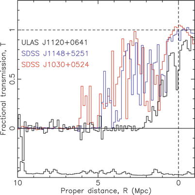
Fig. 10.9
The spectra of three high-redshift QSOs
(SDSS J1148+5251 at z = 6. 42, SDSS J1030+0524 at
z = 6. 31, and the
z = 7. 085 QSO ULAS
J1120+0641) at the Lyman-α
emission line. For this figure, the wavelength difference to the
Lyman-α transition is
expressed in proper distance away from the QSOs. The spectra are
normalized, dividing them by the extrapolation of the continuum on
the red side of the emission line, yielding the transmission.
Source: D.J. Mortlock et al. 2011, A luminous quasar at a redshift of z =
7.085, Nature 474, 616, Fig. 3. Reprinted by permission of
Macmillan Publishers Ltd: Nature, ©2011
However, these highest mass objects are very rare
and, by themselves, by far not able to explain reionization. This
fact can be clearly seen by considering the spectral shape of the
Lyα emission line of
high-redshift QSOs. Figure 10.9 shows the spectrum of three very high
redshift QSOs near to the Lyman-α emission line. Whereas all three QSO
show essentially no flux shortward of Lyman-α, once the wavelength difference
exceeds ∼ 20 Å in the restframe, there is some transmitted flux
very close to the Lyman-α
transition. This near-zone transmission is understood as a region
around the QSO where the intergalactic gas is fully ionized by the
QSO, so it becomes transparent. The figure shows a clear trend that
the size of this near zone decreases for higher redshifts, as would
be expected due to the higher gas density and probably larger mean
neutral fraction in the Universe. Thus, these very luminous objects
are able to reionize the intergalactic medium in their immediate
surroundings, but their effect is constrained to a rather limited
volume. Most of the ionizing photons must come from the far more
numerous lower-mass galaxies, i.e., far less luminous
sources.
The UV-luminosity
function at high redshifts. The large number of LBG
candidates at redshifts z ≳ 7 recently obtained yields
constraints on the luminosity function of galaxies in the
rest-frame ultraviolet regime of the spectrum. As pointed out in
Sect. 9.2.4, for most of them no
spectroscopic confirmation is available, so that each individual
case is burdened with uncertainty. We have an idea of what the
UV-luminosity function looks like for z ≲ 8, as shown in Fig. 9.41, but the star-formation rate
density beyond z ∼ 8 is
still very uncertain, as shown in Fig. 9.57.
Since at such high redshifts, high-mass dark
matter halos were extremely rare, we actually expect that most star
formation at z ∼ 10 occurs
in very low-mass systems which will be very difficult to detect.
Thus, in order to translate the observed luminosity function into a
star-formation rate, large extrapolations towards very
low-luminosity sources are required, burdened with substantial
uncertainties.
The
UV-slope. The radiation we observe from high-redshift
galaxies corresponds to wavelengths longward of the Lyα transition, i.e., at wavelengths
considerably larger than that of ionizing photons. Therefore, to
relate the observed properties to the ionizing power, the spectral
shape needs to be extrapolated to shorter wavelengths.
This extrapolation is done using a power law for
the UV-continuum which is conventionally parametrized as
S λ ∝ λ β . A source with slope
 corresponds to a flat spectrum in S ν , for which the AB-magnitudes
(see Sect. A.4) would be independent of the chosen filter. Hence,
in order to relate the observed flux of sources to their emission
of ionizing photons, the slope β must be known. In principle, a very
young, low-metallicity stellar population can have a hard spectrum
with β ∼ −3, but as soon as
the metallicity increases above
corresponds to a flat spectrum in S ν , for which the AB-magnitudes
(see Sect. A.4) would be independent of the chosen filter. Hence,
in order to relate the observed flux of sources to their emission
of ionizing photons, the slope β must be known. In principle, a very
young, low-metallicity stellar population can have a hard spectrum
with β ∼ −3, but as soon as
the metallicity increases above  or the age of the stellar
population is larger than ∼ 107 yr, the spectrum will
get flatter; of course, any extinction (and related reddening)
leads to an increase of β
as well.
or the age of the stellar
population is larger than ∼ 107 yr, the spectrum will
get flatter; of course, any extinction (and related reddening)
leads to an increase of β
as well.
corresponds to a flat spectrum in S ν , for which the AB-magnitudes
(see Sect. A.4) would be independent of the chosen filter. Hence,
in order to relate the observed flux of sources to their emission
of ionizing photons, the slope β must be known. In principle, a very
young, low-metallicity stellar population can have a hard spectrum
with β ∼ −3, but as soon as
the metallicity increases above or the age of the stellar
population is larger than ∼ 107 yr, the spectrum will
get flatter; of course, any extinction (and related reddening)
leads to an increase of β
as well.In principle, the slope β can be obtained from observing
galaxies in at least two wavebands. For the highest-redshift
sources, that corresponds to bands in the observed near-IR regime.
Unfortunately, even relatively small photometric uncertainties
translate into rather large error bars on β. At present, observations seem to
indicate that the mean value of β is between − 2 and − 2. 5 for
z ∼ 7 galaxies.
The escape
fraction. Even if the extrapolation from the observed
rest-frame UV at λ ∼ 1500 Å
to the ionizing region of λ < 912 Å were accurate, we still
would not know the emission of ionizing photons from these
galaxies. The interstellar medium in these objects is expected to
absorb many of the ionizing photons, before they can escape the
galaxy. The escape fraction f esc is very uncertain, and
any theoretical estimate of it is highly model dependent.
We thus conclude that, using reasonable guesses
(within the current observational constraints) regarding the
UV-luminosity function at high-z, the UV-slope β, and the escape fraction
(f esc ∼ 0. 2,
as is suggested from the properties of z ∼ 3 LBGs), the number density of
ionizing photons emitted from the early galaxies may be sufficient
to explain the reionization of the Universe at z ∼ 10, as suggested by the results
from the CMB anisotropies.
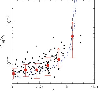
Fig. 10.10
Redshift evolution of the mean neutral
fraction of hydrogen in the intergalactic medium, as obtained from
the absorption of ionizing radiation from high-redshift QSOs
(Gunn–Peterson effect). Individual measurements are shown as
small dots, whereas the
large circles with error
bars represent averages over redshift bins. The two curves show results from numerical
simulations. Source: X. Fan et al. 2006, Constraining the Evolution of the Ionizing
Background and the Epoch of Reionization with z ∼ 6 Quasars. II. A
Sample of 19 Quasars, AJ 132, 117, p. 126, Fig. 7. ©AAS.
Reproduced with permission
Towards a larger
neutral hydrogen fraction.
The observed spectrum of high-redshift QSOs
shortwards of the Lyα
emission line shows that an increasing fraction of the radiation is
absorbed by neutral hydrogen on the line-of-sight. We have seen
that the density of the Lyα
forest increases with redshift (cf. Fig. 10.5) in such a way that
only a tiny fraction of ionizing photons manage to escape
absorption. This observation may be seen as an indication that we
approach the epoch of reionization as the QSO redshift increases
beyond z ∼ 6. However, as
shown in Fig. 10.10, the mean neutral fraction of
intergalactic hydrogen needed to cause this strong absorption of
ionizing photons is still very small—a neutral fraction of much
less than 1 % is sufficient to entirely block the light of QSOs
shortward of the Lyα
emission. Hence, the strong absorption implied by QSO spectra
cannot be taken as evidence for z ∼ 6 signalling the end of the
reionization epoch. Nevertheless, the trend of the data shown in
Fig. 10.10
may suggest that beyond z ∼ 6, we may approach a phase where
the neutral hydrogen fraction indeed starts to increase
significantly.
Observing reionization directly may in principle
be possible if a very high-redshift QSO could be identified whose
absorption spectrum could reveal a tomographic view through the
ionized ‘bubbles’ of the intergalactic medium, as sketched in
Fig. 10.11.
But we point out again that the very dense Lyα forest seen towards QSOs at high
redshift, is no unambiguous sign for approaching the redshift of
reionization, because a very small fraction of neutral atoms (about
1 %) is already sufficient to produce a large optical depth for
Lyα photons.
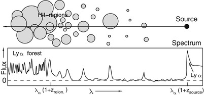
Fig. 10.11
Sketch of a potential observation of
reionization: light from a very distant QSO propagates through a
partially ionized Universe; at locations where it passes through
Hii-regions, radiation
will get through—flux will be visible at the corresponding
wavelengths. When the Hii-regions start to overlap, the
normal Lyα forest will be
produced. Adapted from: R. Barkana & A. Loeb 2000, In the Beginning: The First Sources of Light
and the Reionization of the Universe, astro-ph/0010468
With the upcoming Next Generation Space
Telescope, the James Webb Space Telescope (JWST), one hopes to
observe the epoch of reionization directly and to discover the
first light sources in the Universe; this space telescope, with a
diameter of 6.5 m, will be optimized for operation at wavelengths
between 1 and 5 μm.
10.4 The formation of disk galaxies
We now turn to describe in somewhat more detail
the fate of the cooling gas inside halos. The most important aspect
in addition to the cooling processes described before is the fact
that dark matter halos, and the gas inside of them, contain angular
momentum. As we shall see, this naturally leads to the formation of
galactic disks.
10.4.1 The contraction of gas in halos
We described in Sect. 7.6.2 that a non-spherical
overdensity can attain an angular momentum, due to a torque caused
by the tidal gravitational field in which the overdensity is
located. Therefore, dark matter halos are born with a finite
angular momentum, which we quantified by the spin parameter
λ [see (7.65)]. Analytical estimates and
numerical simulations show that the typical value is λ ∼ 0. 05, however with a rather broad
distribution.
In the initial stages of the evolution of the
overdensity, we expect that baryons and dark matter have the same
spatial distribution, thus the specific angular momentum of the
baryons and dark matter are the same. When the halo collapses, the
gas distribution may become different from that of the dark matter,
but the torque on the halo is strongest at maximum radius (i.e., at
turnaround), and thus during collapse, little angular momentum is
obtained.
When the gas in a halo cools, it collapses toward
the center, thereby conserving its angular momentum. The gas can
therefore not collapse to an arbitrarily small region; the angular
momentum barrier prevents this. Frictional forces in the gas drive
the gas onto approximately circular orbits, depending on the
symmetries of the halo, in a plane perpendicular to the angular
momentum vector—it forms a flat disk. The gas in the disk is much
denser than it would be if the gas retained on almost spherical
distribution; hence, gas in the disk finds it easier to cool and
form stars—in accordance with observations: most of the quiescent
star formation in the current Universe occurs in galactic
disks.
The necessity for
dark matter. Understanding the formation of disk galaxies
requires the presence of dark matter, as we shall see now. Let us
assume the contrary, namely that the density concentration which
formed through gravitational instability consists solely of
baryons. In this case, the baryons are also the only source of
gravity. The characteristic spin parameter of the forming halo is
about 0.05. The spin parameter of a self-gravitating, thin
exponential disk can be calculated to be λ d ≈ 0. 425. As the gas
cloud collapses into a disk, it conserves its mass and its angular
momentum, whereas it can get rid of energy by radiation emitted in
the cooling processes. The binding energy scales like r −1. Therefore, the spin
parameter scales like  , as follows from (7.65). The final spin parameter is
thus related to the initial spin parameter λ i by
, as follows from (7.65). The final spin parameter is
thus related to the initial spin parameter λ i by
 where r i is the
radius of the virialized gas cloud before cooling. In order to get
a spin parameter of ∼ 0. 42 for the exponential disk from a spin
parameter λ i
obtained from tidal torques, the gas must collapse by a
factor ∼ (0. 42∕0. 05)2 ≈ 70.
where r i is the
radius of the virialized gas cloud before cooling. In order to get
a spin parameter of ∼ 0. 42 for the exponential disk from a spin
parameter λ i
obtained from tidal torques, the gas must collapse by a
factor ∼ (0. 42∕0. 05)2 ≈ 70.
, as follows from (7.65). The final spin parameter is
thus related to the initial spin parameter λ i by
(10.11)
We can take our Milky Way as an example for this
process. The radius of the visible disk is of the order of 10 kpc,
which, according to the previous assumptions, would have collapsed
from an initial radius of ∼ 700 kpc. With a baryonic mass of
 for the Milky Way,
the free-fall time from radius 700 kpc is ∼ 4 × 10¹⁰ yr,
i.e., about three times the current age of the Universe. Therefore,
the Milky Way disk could not have formed until today if it
consisted only of baryonic matter. In fact, given that the Milky
Way contains old stars, we have good reasons to assume that it has
formed quite a bit before today, so that the discrepancy of time
scales becomes even stronger.
for the Milky Way,
the free-fall time from radius 700 kpc is ∼ 4 × 10¹⁰ yr,
i.e., about three times the current age of the Universe. Therefore,
the Milky Way disk could not have formed until today if it
consisted only of baryonic matter. In fact, given that the Milky
Way contains old stars, we have good reasons to assume that it has
formed quite a bit before today, so that the discrepancy of time
scales becomes even stronger.Gas collapse in a
dark matter halo. If, however, the gas contracts in a dark
matter halo, the situation is quite different. Assume, for
simplicity, that the density profile of the dark matter halo
behaves like ρ ∝ r −2, up to the virial
radius; this corresponds to the isothermal sphere which we
discussed in Sect. 3.11.2 yielding a
radius-independent rotational velocity V c. If the halo has a spin
parameter of λ = 0. 05,
then the rotational velocity of the halo, and the gas inside of it,
is about V c∕7.
If the gas sinks to the center, thereby conserving its specific
angular momentum ∝ r v, it needs to reduce its radius by a
mere factor of 7 to form a rotationally supported disk—an order of
magnitude less than in the hypothetical case of baryon-only
halos.4 The
time-scale for the formation of a Milky Way-like disk is then
reduced to ∼ 109 yr, thus such disks can form
sufficiently early in the cosmic evolution.
10.4.2 The formation of galactic disks
Empirically, it is found that the light
distribution of disk galaxies follows an exponential law. Assuming
a fixed mass-to-light ratio, this implies that the surface mass
density Σ(R) behaves like
 where Σ 0 is the
central surface mass density, and R d the scale-length of the
disk. For the considerations that follow, we shall assume that the
dark matter in the halo follows an isothermal density profile, and
that the self-gravity of the disk is negligible. The former
assumption is motivated by the observed flat rotation curves of
disk galaxies; we point out that the rotational velocity predicted
by NFW density profiles (see Sect. 7.6.1) is fairly constant over a
broad range of radius.
where Σ 0 is the
central surface mass density, and R d the scale-length of the
disk. For the considerations that follow, we shall assume that the
dark matter in the halo follows an isothermal density profile, and
that the self-gravity of the disk is negligible. The former
assumption is motivated by the observed flat rotation curves of
disk galaxies; we point out that the rotational velocity predicted
by NFW density profiles (see Sect. 7.6.1) is fairly constant over a
broad range of radius.
(10.12)
Estimating the
disk scale length. Starting from a dark matter halo, its
virial mass M, virial
radius r 200 and
virial velocity V
200 are related through (7.58). The assumption of an
isothermal profile then implies that the rotational velocity
V
rot(r) = V 200, independent of
radius, and that the density profile is  . If we assume
that a fraction m
d of the halo mass is contained in the disk, we find for
the disk mass
. If we assume
that a fraction m
d of the halo mass is contained in the disk, we find for
the disk mass

. If we assume
that a fraction m
d of the halo mass is contained in the disk, we find for
the disk mass
(10.13)


where we set  in the last step. In the
isothermal density profile of the dark matter halo, the rotational
velocity of the disk is constant, and so its angular momentum is
in the last step. In the
isothermal density profile of the dark matter halo, the rotational
velocity of the disk is constant, and so its angular momentum is

in the last step. In the
isothermal density profile of the dark matter halo, the rotational
velocity of the disk is constant, and so its angular momentum is
(10.15)
where in the last step we used (10.14). We assume that
the angular momentum of the disk is a fraction j d of the total angular
momentum of the halo, J
d = j
d J
h. The latter can be related to the spin parameter
λ in (7.65), which in addition contains
the total energy of the halo and the halo mass. The total energy
follows from the virial theorem and the simple properties of an
isothermal sphere,  . We then find

. We then find
(10.16)

where we inserted the expression for the binding
energy. Finally, using (7.58) again, this can be written in
the form

(10.18)
Interpretation. This equation contains a
number of interesting aspects. The first expression relates the
virial radius of the halo to the scale-length of the disk. If we
assume that the average specific angular momentum of the gas in the
disk is the same as the average specific angular momentum of the
halo, then j
d = m
d, and we simply get  ; using
the characteristic value of λ ∼ 0. 05, we obtain r 200 ∼ 30R d. For the Milky Way,
R d ≈ 3. 5 kpc,
so that its virial radius is predicted by this consideration to be
about 100 kpc.
; using
the characteristic value of λ ∼ 0. 05, we obtain r 200 ∼ 30R d. For the Milky Way,
R d ≈ 3. 5 kpc,
so that its virial radius is predicted by this consideration to be
about 100 kpc.
; using
the characteristic value of λ ∼ 0. 05, we obtain r 200 ∼ 30R d. For the Milky Way,
R d ≈ 3. 5 kpc,
so that its virial radius is predicted by this consideration to be
about 100 kpc.The final expression in (10.18) relates the virial
velocity—for the assumed isothermal distribution, this is the same
as the rotational velocity—to the scale-length of the disk. Again
using the Milky Way as an example, for which V rot ≈ 220 km∕s, we see
that the predicted scale length is about a factor of two larger
than the observed one, for the same parameters. Thus, although this
simple model provides a result which is within a factor ∼ 2 of the
observed properties of the Milky Way disk, it fails to yield an
accurate quantitative agreement. Of course it is possible that our
Galaxy formed inside a halo where the spin parameter has a rather
low value, or that the disk fraction of angular momentum is
different from its mass fraction. For example, if we keep the
assumption j
d = m
d, a spin parameter of λ ∼ 0. 02 would predict roughly the
correct scale length, but such low values of λ have a rather small probability to
occur. Furthermore, it would also lead to a large virial radius
of ∼ 250 kpc, predicting a very massive halo for the Milky
Way.
However, there is another issue of (10.18) which does not
really fit the observations. The function E(z) at redshift z = 1 is  ,
implying that galactic disks at that epoch are considerably smaller
than those today. Such a strong size evolution of disks is not
consistent with the observations.
,
implying that galactic disks at that epoch are considerably smaller
than those today. Such a strong size evolution of disks is not
consistent with the observations.
,
implying that galactic disks at that epoch are considerably smaller
than those today. Such a strong size evolution of disks is not
consistent with the observations.A third issue with this simple consideration is
the mass fraction of baryons that end up in the disk. With a disk
mass of  for
the Milky Way, (10.13) predicts about m d ∼ 0. 02. If we assume
that the halo contained the same baryon fraction as the cosmic mean
at halo formation, then only about 10 % of the baryons end up in
the disk. As we shall see later, there are processes which prevent
gas from settling down is a disk, but it is difficult to find such
processes efficient enough to hold back 90 % of the baryons.
for
the Milky Way, (10.13) predicts about m d ∼ 0. 02. If we assume
that the halo contained the same baryon fraction as the cosmic mean
at halo formation, then only about 10 % of the baryons end up in
the disk. As we shall see later, there are processes which prevent
gas from settling down is a disk, but it is difficult to find such
processes efficient enough to hold back 90 % of the baryons.Refinements of the
model. The simplified model made a number of assumption
which we know can not be correct in detail: Real dark matter halos
do not have an isothermal profile, but follow approximately an NFW
profile in which the rotational velocity is a slow function of
galactocentric radius. In addition, the contraction of gas changes
the overall gravitational potential of the halo, which also affects
the dark matter distribution; the dark matter also gets somewhat
more concentrated towards the halo center. This halo contraction
will change the rotational velocity further.
The rotation curves of spiral galaxies show that
the neglect of the disk self-gravity is an oversimplification.
Within the optical radius of a disk, the baryons in the disk
contribute substantially to the gravitational field. This is in
accord with what we have learned from gravitational lensing studies
of galaxies which show that within the Einstein radius, about half
the mass is contributed by the baryonic component. Numerical
simulations of disk galaxy formation which take the gas cooling and
halo contraction into account indicate that the rotational velocity
of disks is closely approximated by the maximum rotational velocity
of an NFW profile (see Fig. 7.19) instead of the virial circular
velocity.
Both, inclusion of self-gravity and the halo
contraction lead to larger rotational velocities in the inner part
of the halo compared to the simple model. As a consequence, the
size and mass of the halo is smaller than obtained from the simple
model, so that the corresponding estimate of m d is increased. The proper
inclusion of these two effects also yields a much smaller
redshift-dependence of the scale-length than predicted by
(10.18),
i.e., considerably closer to the observational situation.
We thus conclude that the model described here,
once accounting for the effects of disk self-gravity and halo
contraction, provides a good quantitative model for understanding
the formation of disk galaxies.
10.4.3 Dynamical effects in disks
Once the disk has formed, the gas is sufficiently
dense so that star formation can proceed; we have seen in
Sect. 3.3.3 before that the
Schmidt-Kennicutt law describes the star-formation rate (per unit
disk area) as a function of surface mass density. Hence, after some
time a thin stellar disk is formed, with some fraction of the
baryons left over in the form of gas.
Such a thin disk is subject to dynamical
instabilities. Whereas in an axi-symmetric gravitational potential,
stars move on circular orbits, perturbations of the gravitational
field can perturb these orbits, which in turn can amplify the
deviation from axial symmetry. The formation of spiral arms is one
example of such perturbations. Another important aspect is the
formation of bars in the center of a large fraction of spiral
galaxies. The asymmetry of the bars can yield significant
perturbations of the potential with corresponding changes of
orbits, leading to a redistribution of mass and angular momentum.
In particular, bars can cause stars and gas to migrate inwards,
towards the center.
Pseudo-bulges. The corresponding
accumulation of gas can trigger increased star formation in the
center of galaxies. These stars then form a concentration at the
galactic center. It is generally believed that this is the
mechanism for the formation of pseudo-bulges in spiral galaxies—we
recall that bulges are divided into classical bulges and
pseudo-bulges, the latter being characterized by a Sérsic-index
close to unity and fast rotation, whereas the former ones have a
Sérsic-index close to that of ellipticals and considerably slower
rotation. The formation of classical bulges is thus suspected to be
related to the formation of elliptical galaxies, which will be
discussed below.
Heating of the
stellar distribution. We have seen in Sect. 2.3.1 that the velocity dispersion
of stars in the Milky Way disk depends on their age—the older the
stars, the higher their random velocities. Stars are formed by the
molecular gas which is observed to have the thinnest distribution.
Over their lifetime, the stars can gain a random velocity
component, by scattering on the perturbations of the gravitational
potential, such as caused by giant molecular clouds, spiral arms,
or the subhalo population that we discussed in Sect. 7.8. Whatever the main source of
heating, the trend with stellar age is expected in all these
cases.
10.4.4 Feedback processes
Although the story as told above naturally leads
to the formation of disk galaxies, early studies have shown that
some ingredients are missing. In fact, hydrodynamical simulations
of disk formation show that star formation in the gas disks is far
too efficient, consuming the available gas in too short a time, so
that most of the stars would be formed at high redshift, with
little current star formation left. Furthermore, the resulting
disks are too concentrated and too small, leading to rotation
curves which are declining outwards beyond the (small) half-light
radius of the disk, in marked contrast with observed rotation
curves. This together is known as the overcooling problem in galaxy
evolution. Real disk galaxies have a slower conversion of gas into
stars and their disks remain larger. And finally, the efficient
conversion of gas into stars in our simple model would predict that
the stellar mass density in the Universe is much higher than
observed—whereas Ω
b ∼ 0. 04, the density parameter in stars is less than
1 %. Hence, most baryons in the Universe habe not been converted to
stars.
Feedback by
supernovae. In order to balance the efficient gas cooling,
heating sources need to be considered. An unavoidable source of
heating is the energy injected into the interstellar medium by
supernovae. Very shortly after star formation sets in, the most
massive stars of the stellar population undergo a core-collapse
supernova. The mechanical energy of the explosion is partly
transferred to the gas surrounding the exploding star. Thereby the
gas is heated, causing it to expand, thus to decrease its density,
which in turn reduces its cooling efficiency. Note that this is a
feedback process—the higher the star formation rate, the more
energy is injected into the interstellar gas to prevent, or at
least delay, further star formation. Depending on the efficiency of
this feedback, the local gas of the disk may be blown out of the
disk into the halo (and produce a hot gas corona outside the
disk—see Sect. 3.3.7), or, in particular for
low-mass halos, be removed from the halo through outflowing
gas.
In fact, there is direct observational evidence
of the occurrence of outflows from star-forming galaxies. For
example, we have seen in Sect. 9.1.1 that the spectra of
Lyman-break galaxies reveal substantial mass outflows, at a similar
rate as their star-formation rate and with velocities of several
hundreds of km/s.
The details of this feedback process are somewhat
uncertain—how much of the supernova energy is converted into heat,
and how much is transferred to the interstellar medium in form of
bulk kinetic energy, is not well determined. Furthermore, the
feedback by supernovae depends on the assumed initial mass function
(IMF; see Sect. 3.5.1) of stars, which yields the
fraction of newly formed stars which explode as core-collapse
supernova. The flatter the IMF at the high-mass end, the more
supernova energy per unit mass of newly formed stars is
injected.
Assuming a universal IMF, the energy released by
supernovae per unit mass of newly-formed stars is η SN E SN, where η SN denotes the expected
number of supernovae per unit mass of formed stars, and
E SN is the
energy released per supernova. If we assume that this energy
reheats some of the cold gas back to virial temperature of the
halo, the amount of gas that is reheated after formation of a group
of stars with mass Δ m
∗ is
 where ε parametrizes the
efficiency of the reheating process. The reheated gas may be
transferred back to the hot gaseous halo, whereas other models
assume that the reheated gas is first ejected from the halo, and
only later reincorporated into the hot halo on the dynamical
time-scale of the halo. This ejection scenario effectively delays
the time at which the reheated gas can cool and becomes available
for star formation again.
where ε parametrizes the
efficiency of the reheating process. The reheated gas may be
transferred back to the hot gaseous halo, whereas other models
assume that the reheated gas is first ejected from the halo, and
only later reincorporated into the hot halo on the dynamical
time-scale of the halo. This ejection scenario effectively delays
the time at which the reheated gas can cool and becomes available
for star formation again.
(10.19)
As can be seen from (10.19), supernova
feedback is more efficient at suppressing star formation in
low-mass galaxies—which is due to the fact that the binding energy
per unit mass is an increasing function of halo mass. This simply
expresses the fact that for low-mass halos it is easier to drive
the gas outwards.
AGN
feedback. Whereas supernova feedback explains a decreasing
conversion of gas into stars with decreasing halo mass, and thus
can account for the difference of the slopes between the galaxy
luminosity function and the halo mass function at the low
mass/luminosity end (see Fig. 10.2), it is less efficient for higher-mass
halos, due to the larger V
200 in (10.19). The increase of the cooling time for
higher-mass halos (see Fig. 10.4) by itself cannot account for the abrupt
exponential decrease of the galaxy luminosity function beyond
L ∗. One
requires another process which delays the cooling of gas in
high-mass halos.
For very massive halos, we have already
encountered such a process: The suppression of cooling flows in
galaxy clusters is due to AGN activity of the central galaxy in the
cluster. Since (almost) all massive galaxies contain a supermassive
black hole (see Sect. 3.8), this kind of feedback may be
operational not only in groups and clusters, but actually in
individual massive galaxies as well. In particular, there is a
great deal of evidence for a relation between nuclear starbursts in
galaxies and AGN activity. The gas needed for a starburst in the
center of a galaxy is also potential fuel for the central black
hole. Again, the details of this process are quite uncertain, but
with plausible prescriptions, the cut-off of the luminosity
function at L ≳ L
∗ can be successfully modeled.
Feedback by an AGN can occur in several ways. In
the case of galaxy clusters, the major effect of the AGN is the
insertion of hot bubbles into the intracluster medium through radio
jets. The AGNs in most central cluster galaxies are not very
luminous, and seem to be in the ‘radio mode’ (see
Sect. 5.5.5) of low accretion rate. Thus,
for low accretion rates, the main channel of feedback is the
injection of mechanical energy into the surrounding gas. At high
accretion rates, in the ‘quasar mode’, the main source of feedback
is presumably heating of the gas. Furthermore, the strong radiation
field from quasars changes the ionization structure of the
surrounding gas, which affects its cooling curve compared to the
one shown in Fig. 10.3 and at low temperatures actually leads to
radiative heating. These various effects should be included in
realistic models of the evolution of galaxies, at least in an
approximate way; we shall come back to this below.
10.4.5 The formation and evolution of supermassive black holes
Black holes grow in mass by accreting material, a
process we witness through the radiation from accreting black holes
in AGNs (Chap. 5). Hence, once a population of
supermassive black holes (SMBHs) is present, their evolution can be
studied observationally, as well as through modeling. But how did
the first generation of SMBH form? There is no firm conclusion on
this question, but three plausible formation processes have been
studied in detail. What we do know, however, is that the first
SMBHs must have formed very early in the Universe, as indicated by
the presence of very luminous QSOs at z > 6.
Remnants of
population III stars. The first stars in the Universe form
out of primordial gas, i.e., gas with zero metallicity. The cooling
properties of this gas are quite different from those of enriched
material, since no metal lines are available for radiating energy
away. From simulations of star formation in primordial gas, it is
suggested that many stars can form with very high masses, well
above  . These stars burn their nuclear fuel
very quickly, in a few million years, before they end their lives
explosively. If the mass of a star is above
. These stars burn their nuclear fuel
very quickly, in a few million years, before they end their lives
explosively. If the mass of a star is above  , its supernova will leave a
black hole behind with a mass of
, its supernova will leave a
black hole behind with a mass of  . Since the first stars are
expected to form at
. Since the first stars are
expected to form at  , this formation mechanism would yield
a very early population of seed black holes. However, it is still
unknown whether such very massive population III stars indeed
formed.
, this formation mechanism would yield
a very early population of seed black holes. However, it is still
unknown whether such very massive population III stars indeed
formed.
. These stars burn their nuclear fuel
very quickly, in a few million years, before they end their lives
explosively. If the mass of a star is above , its supernova will leave a
black hole behind with a mass of . Since the first stars are
expected to form at , this formation mechanism would yield
a very early population of seed black holes. However, it is still
unknown whether such very massive population III stars indeed
formed.Gas-dynamical
processes. Another route for the formation of supermassive
black holes arises if the primordial gas in a high-redshift dark
matter halo manages to concentrate in its center, through global
dynamical instabilities (e.g., related to the formation of bar-like
structures) that are able to transport angular momentum outwards.
This angular momentum transport is needed since otherwise, the
central concentration of gas would be prevented by the angular
momentum barrier. Subsequent cooling by molecular hydrogen may then
lead to the formation of a rapidly rotating supermassive star with
up to  , provided the accumulation of the
gas occurs rapidly enough. Once the inner core of this supermassive
star has burned its hydrogen, the core will collapse and form a
black hole with a few tens of
, provided the accumulation of the
gas occurs rapidly enough. Once the inner core of this supermassive
star has burned its hydrogen, the core will collapse and form a
black hole with a few tens of  , where this mass depends on the initial
angular velocity of the star. This black hole subsequently accretes
material from the outer layers of the star, and this
quasi-spherical accretion has a very low radiative efficiency
ε. Therefore, the black
hole can grow in mass quickly, until finally its exceeds the
Eddington luminosity and the remaining gas is expelled, leaving
behind a SMBH with
, where this mass depends on the initial
angular velocity of the star. This black hole subsequently accretes
material from the outer layers of the star, and this
quasi-spherical accretion has a very low radiative efficiency
ε. Therefore, the black
hole can grow in mass quickly, until finally its exceeds the
Eddington luminosity and the remaining gas is expelled, leaving
behind a SMBH with  .
.
, provided the accumulation of the
gas occurs rapidly enough. Once the inner core of this supermassive
star has burned its hydrogen, the core will collapse and form a
black hole with a few tens of , where this mass depends on the initial
angular velocity of the star. This black hole subsequently accretes
material from the outer layers of the star, and this
quasi-spherical accretion has a very low radiative efficiency
ε. Therefore, the black
hole can grow in mass quickly, until finally its exceeds the
Eddington luminosity and the remaining gas is expelled, leaving
behind a SMBH with .Stellar-dynamical
processes. In the inner part of a forming galaxy, dense
nuclear star clusters may form. Because of the high density,
star-star collisions can occur which can lead to the formation of
very massive stars with mass exceeding  . This has to happen very quickly,
before the first stars explode as supernovae, since otherwise the
massive star would be polluted with metals, its opacity increased,
and it would no longer be stable. The fate of this supermassive
star is then similar to the scenario described above, resulting in
a black hole remnant of several hundred Solar masses.
. This has to happen very quickly,
before the first stars explode as supernovae, since otherwise the
massive star would be polluted with metals, its opacity increased,
and it would no longer be stable. The fate of this supermassive
star is then similar to the scenario described above, resulting in
a black hole remnant of several hundred Solar masses.These three possibilities are not mutually
exclusive. At present, our theoretical understanding of these
processes is not sufficient to establish their likelihood of
occurrence. Whereas one may be able to distinguish between these
scenarios, e.g., from the statistics of black hole masses in
present day low-mass galaxies, the current observational situation
does not conclusively support or reject any of these three
routes.
Mass
growth. Once the seed black holes have formed, they can grow
in mass by accreting material. We saw in Sect. 5.3.5 that the characteristic
time-scale for mass growth, i.e., the time on which the black hole
mass can double, is  .
With ε ∼ 0. 1, a
.
With ε ∼ 0. 1, a
 seed black hole formed at
z ∼ 20 could grow to a
seed black hole formed at
z ∼ 20 could grow to a
 by redshift 7
if it accreted continuously at the Eddington rate. The situation is
more difficult for seed black holes formed from population III
stars; they probably require super-Eddington accretion rates to be
able to power the luminous QSOs at z > 6. As mentioned in
Sect. 5.3.5, the accretion rate may
exceed the Eddington rate though probably not by a large
factor.
by redshift 7
if it accreted continuously at the Eddington rate. The situation is
more difficult for seed black holes formed from population III
stars; they probably require super-Eddington accretion rates to be
able to power the luminous QSOs at z > 6. As mentioned in
Sect. 5.3.5, the accretion rate may
exceed the Eddington rate though probably not by a large
factor.
.
With ε ∼ 0. 1, a
seed black hole formed at
z ∼ 20 could grow to a
by redshift 7
if it accreted continuously at the Eddington rate. The situation is
more difficult for seed black holes formed from population III
stars; they probably require super-Eddington accretion rates to be
able to power the luminous QSOs at z > 6. As mentioned in
Sect. 5.3.5, the accretion rate may
exceed the Eddington rate though probably not by a large
factor.10.4.6 Cosmic downsizing
The hierarchical model of structure formation
predicts that smaller-mass objects are formed first, with more
massive systems forming later in the cosmic evolution. As discussed
before, there is ample evidence for this to be the case; e.g.,
galaxies are in place early in the cosmic history, whereas clusters
are abundant only at redshifts z ≲ 1. However, looking more closely
into the issue, apparent puzzles are discovered. For example, the
most massive galaxies in the local Universe, the massive
ellipticals, contain the oldest population of stars, although at
first sight, their formation should have occurred later than those
of less massive galaxies. In turn, most of the star formation in
the local Universe seems to be associated with low- or
intermediate-mass galaxies, whereas the most massive ones are
passively evolving. Now turning to high redshift: for z ∼ 3, the bulk of star formation seems
to occur in LBGs and SMGs, which, according to their clustering
properties (see Sect. 9.1.1), are associated with
high-mass halos. The study of passively evolving EROs indicates
that massive old galaxies were in place as early as z ∼ 2, hence they must have formed very
early in the cosmic history. The phenomenon that massive galaxies
form their stars in the high-redshift Universe, whereas most of the
current star formation occurs in galaxies of lower mass, has been
termed ‘downsizing’. We saw in Sect. 5.6.2 that a similar phenomenon
also is observed for AGNs.
This downsizing can be studied in more detail
using redshift surveys of galaxies. The observed profile of the
absorption lines in the spectra of galaxies yields a measure of the
characteristic velocity and thus the mass of the galaxies (and
their halos). Studies carried out in the local Universe showed that
local galaxies have a bimodal distribution in color (see
Sect. 3.1.3), which in turn is related to
a bimodal distribution in the specific star-formation rate.
Extending such studies to higher redshifts, by spectroscopic
surveys at fainter magnitudes, we can study whether this bimodal
distribution changes over time. In fact, such studies reveal that
the characteristic mass separating the star-forming galaxies from
the passive ones evolves with redshift, such that this dividing
mass increases with z. For
example, this characteristic mass decreased by a factor of ∼ 5
between z = 1. 4 and
z = 0. 4. Hence, the mass
scale above which most galaxies are passively evolving decreases
over time, restricting star formation to increasingly lower-mass
galaxies.
Studies of the fundamental plane for field
ellipticals at higher redshift also point to a similar conclusion.
Whereas the massive ellipticals at z ∼ 0. 7 lie on the fundamental plane
of local galaxies when passive evolution of their stellar
population is taken into account, normal ellipticals of lower mass
at these redshifts have a smaller mass-to-light ratio, indicating a
younger stellar population. Also here, the more massive galaxies
seem to be older than less massive ones. To reproduce these
evolutionary effect requires to account for AGN feedback in models
of galaxy evolution.
10.5 Formation of elliptical galaxies
Properties of
ellipticals. Whereas the formation of disk galaxies can be
explained qualitatively in a relatively straightforward way, the
question of the formation of ellipticals is considerably more
difficult to answer. Stars in ellipticals feature a high velocity
dispersion, indicating that they were not formed inside a cool gas
disk, or that the stellar distribution was subsequently heated very
strongly. On the other hand, it is hard to comprehend how star
formation may proceed without gas compression induced by
dissipation and cooling.
In Sect. 3.4.3 we saw that the properties of
ellipticals are very well described by the fundamental plane. It is
also found that the evolution of the fundamental plane with
redshift can almost completely be explained by passive evolution of
the stellar population in ellipticals. In the same way, we stated
in Sect. 6.8 that the ellipticals in a
cluster follow a very well-defined color-magnitude relation (the
red cluster sequence), which suggests that the stellar populations
of ellipticals at a given redshift all have a similar age. By
comparing the colors of stellar populations in ellipticals with
models of population synthesis, an old age for the stars in
ellipticals is obtained, as shown in Fig. 3.35
Monolithic
collapse. A simple model is capable of coherently describing
these observational facts, namely the monolithic collapse.
According to this description, the gas in a halo is nearly
instantaneously transformed into stars. In this process, most of
the gas is consumed, so that no further generations of stars can
form later. For all ellipticals with the same redshift to have
nearly identical colors, this formation must have taken place at
relatively high redshift, say z ≳ 2, so that the current ellipticals
are all of essentially the same age. This scenario thus requires
the formation of stars to happen quickly enough, before the gas can
accumulate in a disk. The process of star formation remains
unexplained in this picture, however, and most likely this model
does not describe the processes that are responsible for the
formation of ellipticals.
Instead, we have very good reasons to believe
that elliptical galaxies form as a consequence of galaxy
transformations. For example, we have seen that most ellipticals
are found in dense environments, like groups and clusters, and
within these high-mass structures, they are concentrated towards
their center. In other words, elliptical galaxies are located in
regions where, due to the enhanced density, interactions of
galaxies happen preferentially. Furthermore, elliptical galaxies
have rather complicated kinematics, often exhibiting small disks
(sometimes counter-rotating) around their center, shells and
ripples, which indicate a lively history of these objects. From a
theoretical view, hierarchical structure formation predicts that
high-mass halos are formed by merging of smaller ones, and so the
collision of halos and their embedded galaxies must play a role in
the distribution of galaxy properties. We shall therefore take a
closer look at such halo mergers.
10.5.1 Merging of halos and their galaxies.
When two halos merge to form one with larger
mass, their baryonic components will be affected as well. We have
seen spectacular examples of this process in the form of colliding
galaxies (e.g., Fig. 1.16). Clearly, after the two spiral
galaxies collided, the resulting stellar distribution does not
resemble that of a spiral anymore. Mergers of halos, and associated
collision of galaxies, lead to morphological transformation of
galaxies. Furthermore, such galaxy collisions are generally
accompanied by massive star bursts. Hence, also the stellar
population of the resulting object is affected by collisions.
In the Antennae (see Fig. 9.25), the mass of the two galaxies
which collide is about equal. However, one expects that the
collision of galaxies with very different masses is more frequent,
and such mergers will have different consequences for the
respective galaxies. One thus distinguishes between minor mergers, where the mass ratios of
halos is large (typically in excess of 3:1), and major mergers
where the two masses are similar.
Conditions for
merging. Not every (near) collision of two halos leads to a
merger. For example, we have seen in the bullet cluster
(Sect. 6.6.2) that the two clusters simply
move through each other, since their dark matter and stellar
components are collisionless. Only the (collisional) gas components
of the two clusters are strongly affected by this collision, but no
merging will take place. The reason is that the relative velocity
of these two clusters at collision is much larger than their
internal velocity dispersion, or expressed differently, that the
collision speed is much higher than the escape velocity of each
cluster component.5
In order for a merger to happen, the collisional speed has to be of
the same order, or smaller, than the intrinsic velocity dispersion.
This implies that effective mergers of galaxies do not occur in
massive clusters, where the velocity dispersion of the galaxies of
the cluster—which is also the characteristic collision velocity—is
considerably higher than the stellar velocity dispersion of the
individual galaxies. In contrast, groups of galaxies have both, a
high density of galaxies making collisions probable, and a
sufficiently low velocity dispersion to enable the merging of
galaxies. Hence we expect that the most efficient merging of
galaxies happens in groups.
Minor
mergers. Consider what may happen in the merging of two
halos with their embedded galaxies. The outcome of a merger depends
on several parameters, like the relative velocity, the impact
parameter, the angular momenta, the orientation of their rotation,
and particularly the mass ratio of the two merging halos. If a
smaller galaxy merges with a massive one, the properties of the
dominating galaxy are expected to change only marginally: the small
galaxy will be embedded into the bigger halo, and survive as a
satellite galaxy for a long while. Examples of this are the
Magellanic Clouds, which orbit around the center of the Milky Way
in its dark matter halo. Depending on the orbit of the satellite
galaxy, it will not survive forever. Tidal forces strips matter
from the outer parts of the satellite’s dark halo, which is thus
expected to lose mass—the closer it orbits near the center, the
stronger the tidal forces, and thus the higher the mass-loss
rate.
Dynamical friction (see Sect. 6.3.3) acts on the satellite,
causing it to lose orbital energy and angular momentum, which is
transferred (mostly) to the dark matter halo of the massive
collision partner. The satellite slowly migrates towards the
center, and gets disrupted due to the stronger tidal forces there.
The stars of the satellite galaxy are simply added to the stellar
population of the massive galaxy, since the stars of the satellite
have a small velocity dispersion, they are added as coherent
‘streams’ to the main galaxy (see Fig. 3.17). Such a ‘minor merger’ is
currently taking place in the Milky Way, where the Sagittarius
dwarf galaxy is being torn apart by the tidal field of the Galaxy,
and its stars are being incorporated into the Milky Way as an
additional population. This population has, by itself, a relatively
small velocity dispersion, forming a cold stream of stars that can
also be identified as such by its kinematic properties. However,
the large-scale structure of the Galaxy is nearly unaffected by a
minor merger like this.
The thick disk and
the stellar halo. Spiral galaxies have, beside the thin
stellar and gas disk, also a thick disk with distinct properties:
it has a substantially larger scale-height (by a factor of ∼ 3) and
a stellar population with lower metallicity and old age. Thick
disks have been explained by a number of different models. For
example, they could consist of stars formed in the thin disk, and
being heated so strongly that their vertical velocity dispersion
causes this population to thicken substantially. However, the
clearly different age distribution of thick-disk stars provides an
obstacle for this explanation which rather predicts a continuous
transition from thin to thick-disk stars. Nevertheless, the
satellite galaxies and their associated subhalos may well be a
substantial source of heating.
Minor mergers provide an alternative explanation
for the origin of thick disks. Due to dynamical friction, satellite
galaxies are dragged into the plane of the disk of the parent
galaxy, and their subsequent disruption leaves their stars in the
plane of the disk. As the minor merger partner is of low mass, the
age of the thick disk is expected to be old—we have seen that
low-mass halos preferentially form their stars very early in cosmic
history, before heating by an ionizing background radiation
prevents efficient star formation. It is thus conceivable that the
stars of the thick disk, and also those of the stellar halo, are
relics of earlier minor mergers. The fact that an increasing number
of stellar streams are found in the Milky Way and other neighboring
galaxies, as well as numerical simulations, support this
picture.
Thus, in summary, minor mergers do not alter the
properties of the major collision partner strongly. The dark matter
halo increases its mass, in the form of subhalos (which later on
may be disrupted), the stellar population of the low-mass galaxy
first forms a satellite galaxy, which later can be disrupted and
added to the stellar population of the parent galaxy, probably with
somewhat different kinematical properties.
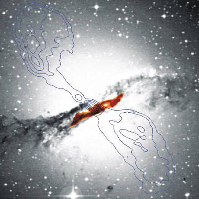
Fig. 10.12
The galaxy Centaurus A. The optical image
is displayed in grayscales, the contours show the radio emission,
and in red, an infrared
image is presented, taken by the ISO satellite. The ISO map
indicates the distribution of dust, which is apparently that of a
barred spiral. It seems that this elliptical galaxy features a
spiral that is stabilized by the gravitational field of the
elliptical. Presumably, this galaxy was formed in a merger process;
this may also be the reason for the AGN activity. Credit: ESA/ISO,
ISOCAM Team, I.F. Mirabel and O. Laurent (CEA/DSM/DAPNIA),
et al. 1998, astro-ph/9810419
Major mergers and
morphological transformations of galaxies. The situation is
different in a merger process where both partners have a comparable
mass. In such ‘major mergers’ the galaxies will change completely.
The disks will be destroyed, i.e., the disk population attains a
high velocity dispersion and can transform into a spheroidal
component. Furthermore, the gas orbits are perturbed, which may
trigger massive starbursts like, e.g., in the Antenna galaxies. By
means of this perturbation of gas orbits, the SMBH in the centers
of the galaxies can be fed, initiating AGN activity, as it is
presumably seen in the galaxy Centaurus A shown in
Fig. 10.12.
Due to the violence of the interaction, part of the matter is
ejected from the galaxies. These stars and the respective gas are
observable as tidal tails in optical images or by the 21 cm
emission of neutral hydrogen. From these arguments, which are also
confirmed by numerical simulations, one expects that in a ‘major
merger’ an elliptical galaxy may form. In the violent interaction,
the gas is either ejected, or heated so strongly that any further
star formation is suppressed.
Dry vs. wet
mergers. However, the situation is slightly more complicated
than this. The violent starbursts, associated with the collision of
gas-rich galaxies, generate a population of newly-born stars. If
such mergers happen at redshifts z ≲ 2, the stellar population of the
resulting galaxy may not resemble the ‘dead and red’ properties of
observed ellipticals. Therefore, if ellipticals are formed through
major mergers of gas-rich galaxies, that had to happen at an early
epoch. One often calls the mergers where the two progenitor
galaxies are gas-rich ‘wet’ mergers, and contrasts them to ‘dry’
mergers where gas plays only a small role.
Besides the issue of star formation, wet mergers
are characterized by the dissipational properties of the gas. The
associated friction can lead to higher spatial densities than it is
possible for collisionless matter only. The gas can be driven
towards the center of the merger remnant, condense there and form
new stars. This process increases the matter density relative to
the case of dry mergers.
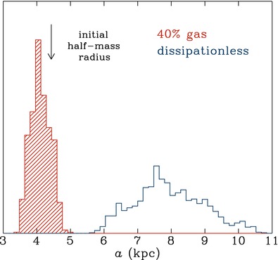
Fig. 10.13
Resulting distribution of the (half-light)
semi-major axis a of merger
remnants. The merging of identical disk galaxies was simulated,
using a distribution of initial conditions, concerning orbital
parameter and orientation of the disks. The merger remnants have
fairly elliptical isophotes. Two families of simulations were
considered: in the first one, the stellar disk of the progenitor
galaxies consisted only of stars (dissipationless), whereas for the
second family, a gas fraction of 40 % was assumed. The figure shows
that the stellar distributions from dissipationless merger remnants
have a rather large size, considerably larger than elliptical
galaxies (the arrow
indicates the half-mass radius of the progenitor disks). The
inclusion of gas and corresponding cooling and star formation
drastically changes this distribution towards considerably smaller
sizes, in agreement with observations. Source: T.J. Cox et al.
2006, The Kinematic Structure of
Merger Remnants, ApJ 650, 791, p. 795, Fig. 3. ©AAS.
Reproduced with permission
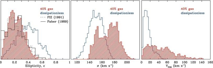
Fig. 10.14
From the same simulations as those
described in Fig. 10.13, the distribution of ellipticity
(left panel), central
velocity dispersion (middle) and maximum velocity along the
major axis (right) are
shown. In each panel, the blue
curves are from the dissipationless simulations, whereas for
the red hatched histograms,
gas physics was taken into account. The black curve in the left panel depicts
the observed distribution of galaxy ellipticities. Source: T.J. Cox
et al. 2006, The Kinematic
Structure of Merger Remnants, ApJ 650, 791, p. 795, Fig. 3.
©AAS. Reproduced with permission
Early numerical simulations of galaxy mergers
considered just the collisionless matter. Although the merger
remnants resembled elliptical galaxies in many respects, in detail
they differed from real ellipticals. For example, the resulting
sizes were considerably larger than those of ellipticals (see
Fig. 10.13).
However, when merger simulations including gas physics became
possible, the situation changed drastically. As we can see from
Fig. 10.13,
the inclusion of gas leads to considerably more concentrated merger
remnants, in accord with observed properties of ellipticals. This
is because the gas condenses in the central region of the merger
remnant and forms stars there, yielding a higher mass (and stellar)
concentration. Furthermore, as illustrated in Fig. 10.14, the distribution
of the ellipticities of the stellar distribution in the remnant is
changed significantly and much better resembles that found in
observations. Wet mergers lead to considerably larger rotational
velocities and central velocity dispersions than dry mergers, again
in agreement with observations.
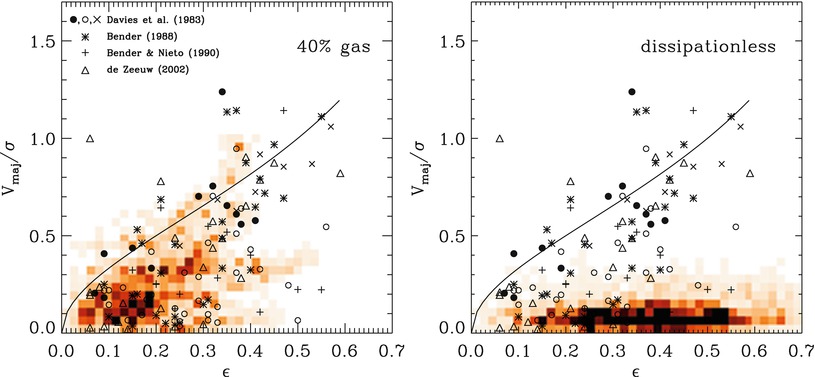
Fig. 10.15
Based on the same simulations as in
Fig. 10.13,
the distribution of the merger remnants in the parameter plane
spanned by the ratio of the maximum rotational velocity along the
major axis and the mean velocity dispersion within the half-light
radius, and the ellipticity of the half-light ellipse of the
stellar distribution of the merger remnant is shown as shaded areas. The left panel includes gas physics,
whereas the right panel
shows the dissipationless mergers. The curves in each panel shows the velocity
ratio that would be needed to cause the flattening of ellipticals
due to rotational support. Overplotted are the corresponding
quantities of several samples of elliptical galaxies. Source: T.J.
Cox et al. 2006, The
Kinematic Structure of Merger Remnants, ApJ 650, 791,
p. 797, Fig. 5. ©AAS. Reproduced with permission
A further strong difference between dry and wet
mergers is the distribution of merger remnants with regards to
their ratio of rotational velocity and velocity dispersion, and the
projected ellipticity of the stellar light. We infer from
Fig. 10.15
that dry mergers of disk galaxies predict far too small rotation of
ellipticals when compared to observations, whereas wet mergers
astonishingly well reproduce the observed distribution. Simulations
like these therefore yield strong support for the merger hypothesis
as the origin of elliptical galaxies. The required high gas
fraction of the disk is a natural consequence of the requirement
that these wet mergers have to happen early in cosmic history, to
reproduce the old stellar population of current ellipticals. At
high redshift, a smaller fraction of the gas has yet been converted
into stars; thus, high-redshift disks are expected to be more gas
rich than current spiral galaxies. Indeed, we saw in
Sect. 9.4.4 that the gas-mass fraction of
high-redshift galaxies is considerably higher than that of local
ones.
Still, this is not the full story. Whereas the
properties of ‘normal’ elliptical galaxies are well reproduced by
the aforementioned gas-rich merger simulations, they fail to
account for some of the characteristics of massive ellipticals,
namely that these are slowly rotating and have boxy isophotes. Such
objects, on the other hand, are produced by (dry) mergers of
ellipticals.
The resulting
scenario for the formation of ellipticals. Therefore, the
following picture emerges: lower-mass normal ellipticals (i.e., not
including dwarfs) are formed by wet major mergers of gas-rich
(disk) galaxies at high redshift. Such mergers preferentially occur
in overdense regions, i.e., in galaxy groups, which explains why
ellipticals are preferentially found in groups and galaxy clusters
(clusters are mainly formed by merging and accretion of groups,
together with the galaxies they contain). In these dense
environments, some of the ellipticals merge with other ellipticals,
and these dry mergers lead to the formation of more massive
galaxies with the characteristics of observed massive
ellipticals.6
Numerical simulations have shown that gas-free
mergers preserve the fundamental plane, in the sense that the
merging of two ellipticals that live on the fundamental plane will
lead to a merger remnant that lies on the plane as well.
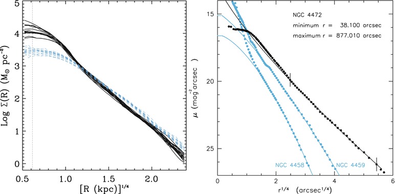
Fig. 10.16
The left
panel shows the radial density profile of merger remnants,
obtained from the gas-rich (black) and dissipationless
(blue) merger simulations
that were also considered in the previous figures. The right panel shows the corresponding
radial surface brightness distribution of three elliptical galaxies
in the Virgo cluster. The black
points correspond to NGC 4472, a core elliptical, with the
best fitting Sérsic profile shown as black curve. The angular region over
which this fit was obtained is indicated by the short vertical lines. The two sets of
blue points and
curves show the brightness
profiles of NGC 4458 and NGC 4459 and the best Sérsic profile fits
at large radii, respectively. Source: Left: T.J. Cox et al. 2006,
The Kinematic Structure of Merger
Remnants, ApJ 650, 791, p. 796, Fig. 4. ©AAS. Reproduced
with permission. Right: J.
Kormendy et al. 2009, Structure and Formation of Elliptical and
Spheroidal Galaxies, ApJS 182, 216, p. 274, Fig. 49. ©AAS.
Reproduced with permission
Brightness
profiles of merger remnants. Support for this picture comes
from the brightness profiles of elliptical galaxies. The left panel
in Fig. 10.16
shows the surface density profile of stars in the merger remnants.
At large radii, they seem to be well described by a de Vaucouleurs
profile (or, more generally, by a Sérsic profile), but there are
significant differences closer to the center. The profiles of the
dissipationless merger remnants near the center lie significantly
below the extrapolation of the de Vaucouleurs profile from larger
radii—these profiles have developed a finite core. On the other
hand, the density of gas-rich merger remnants is higher in their
center than the de Vaucouleurs extrapolation, which can be
accounted for by the increased density through the star formation
in wet mergers.
Interestingly enough, these two kinds of behavior
are also found in elliptical galaxies. In a complete census of all
known elliptical galaxies in the Virgo cluster, it was found that
all the ten brightest
galaxies have a core; one example is NGC 4472 shown in the right
panel of Fig. 10.16. All of the 17 least luminous normal
ellipticals have an excess of light above the extrapolation of the
fitted Sérsic profile; two such examples are also shown in
Fig. 10.16.
The excess light can be explained by the gas dissipation and star
formation in wet mergers, whereas dry mergers are not expected to
develop such a light excess.
This picture is also supported further by the
strong size evolution of elliptical galaxies with redshift (see
Fig. 9.47). An elliptical which formed at
high redshift by a wet merger is more compact than one which is the
result of a dry merger at lower redshift (see Fig. 10.13). Additionally, the
fact that the total stellar mass in massive elliptical galaxies is
smaller by a factor ∼ 3 at z ∼ 1 than today implies that most of
the current ellipticals have formed rather recently—however, not
their stellar population which is required to be old. Such an
evolution of the population of ellipticals can at least be
qualitatively understood with the hypothesis of dry mergers.
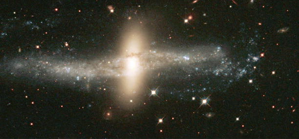
Fig. 10.17
An HST image of NGC 4650A, one out of about
100 known polar-ring galaxies. Spectroscopy shows that the inner
disk-like part of the galaxy rotates around its minor axis. This
part of the galaxy is surrounded by a rotating ring of stars and
gas which is intersected by the polar axis of the disk. Hence, the
inner disk and the polar ring have angular momentum vectors that
are pretty much perpendicular to each other; such a configuration
cannot form from the ‘collapse’ of the baryons in a dark matter
halo. Instead, the most probable explanation for the formation of
such special galaxies is a huge collision of two galaxies in the
past. Originally the disk may have been the disk of the more
massive of the two collision partners, whereas the less massive
galaxy has been torn apart and its material has been forced into a
polar orbit around the more massive galaxy. New stars have then
formed in the disk, visible here in the bluish knots of bright
emission. Since the polar ring is deep inside the halo of the other
galaxy, the halo mass distribution can be mapped out to large radii
using the kinematics of the ring. Credit: J. Gallagher & the
Hubble Heritage Team (AURA/STScI/NASA)
Evidence for the importance of mergers for
ellipticals is also provided by their small-scale brightness
structure. We have seen in Sect. 3.2.5 that many ellipticals show
signs of complex evolution which can be interpreted as the
consequence of mergers. This is in accord with the picture where
the formation of ellipticals in galaxy groups happens by violent
merger processes, and that these then contribute to the cluster
populations by the merging of groups into clusters.
The rate of mergers can be roughly estimated from
the number of close pairs of galaxies with the same redshift. An
example of this is found in Fig. 6.68, where several gravitationally
bound pairs of early-type galaxies are seen in the outskirts of a
cluster at z = 0. 83. These
pairs will merge on a time-scale of ≲ 1 Gyr.
Whereas the impact of a major merger on the fate
of a galaxy is dramatic, these events are not the primary process
by which galaxies obtain their mass. Most of the mass growth of
dark matter halos occurs through minor mergers and accretion of
surrounding material, with major mergers contributing at
the ∼ 20 % level. Indeed,
from the large population of disk galaxies in the current Universe
one concludes that at least for them, major mergers have played no
role in the more recent cosmic history.
Polar ring
galaxies. Another class of particular galaxies may provide
the clearest indication of a merging process for their formation:
polar ring galaxies (see Fig. 10.17). The kinematics of their stellar
population cannot be explained by the collapse of gas in a halo,
but must be due to an encounter of two galaxies.
The impact of AGN
feedback in mergers. The black holes in the center of
galaxies can be switched to an active mode if gas can be channeled
into the center and subsequently accreted. Due to the angular
momentum of gas, this is possible only if the gravitational field
is substantially perturbed, either by internal processes in a
galaxy (e.g., the presence of a bar), or external perturbations.
Indeed, observations of low-redshift QSOs show that they are
preferentially found in host galaxies which show signs of tidal
interactions. It is therefore natural to expect that AGN activity
is promoted by galaxy interactions, in particular by mergers.
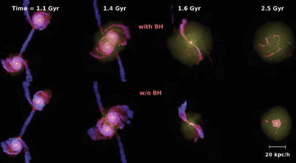
Fig. 10.18
Four different stages of a simulated
merging event of two spiral galaxies whose dark matter halos have a
virial velocity of 160 km∕s. The galaxies also have a stellar bulge
and a gas-mass fraction in the disk of 20 %. The top panel shows the case that both
galaxies contain a supermassive black hole with an initial mass of
 , whereas no SMBHs are
included in the lower
panel. A radiative efficiency of 10 % is assumed for the
black hole accretion, and that 5 % of this energy can be
transferred to heating the gas. In both cases, the gas distribution
is shown, and color
indicates gas temperature, increasing from blue to red to yellow.
After their first mutual passage (the first time step shown), the
two galaxies show strong signs of interactions, as seen in the
tidal tails they develop. Shortly before they merge (second time
step), the gas is considerably hotter in the case where SMBHs are
included—it is heated by the energy from the AGN. The difference
becomes even larger in the later stages of the merging: in the
simulation with SMBHs, the gas density is low and heated to a high
temperature, so that further star formation in the merger remnant
is strongly suppressed: it resembles an early-type galaxy. During
the merger, the accretion of gas is very efficient, and the final
black hole mass of the merger remnant is
, whereas no SMBHs are
included in the lower
panel. A radiative efficiency of 10 % is assumed for the
black hole accretion, and that 5 % of this energy can be
transferred to heating the gas. In both cases, the gas distribution
is shown, and color
indicates gas temperature, increasing from blue to red to yellow.
After their first mutual passage (the first time step shown), the
two galaxies show strong signs of interactions, as seen in the
tidal tails they develop. Shortly before they merge (second time
step), the gas is considerably hotter in the case where SMBHs are
included—it is heated by the energy from the AGN. The difference
becomes even larger in the later stages of the merging: in the
simulation with SMBHs, the gas density is low and heated to a high
temperature, so that further star formation in the merger remnant
is strongly suppressed: it resembles an early-type galaxy. During
the merger, the accretion of gas is very efficient, and the final
black hole mass of the merger remnant is  . In the simulation
without SMBHs, a substantial amount of cool gas remains to enable
ongoing star formation. Source: T. di Matteo et al. 2005,
Energy input from quasars
regulates the growth and activity of black holes and their host
galaxies, Nature 433, 604, Fig. 1. Reprinted by permission
of Macmillan Publishers Ltd: Nature, ©2005
. In the simulation
without SMBHs, a substantial amount of cool gas remains to enable
ongoing star formation. Source: T. di Matteo et al. 2005,
Energy input from quasars
regulates the growth and activity of black holes and their host
galaxies, Nature 433, 604, Fig. 1. Reprinted by permission
of Macmillan Publishers Ltd: Nature, ©2005
, whereas no SMBHs are
included in the lower
panel. A radiative efficiency of 10 % is assumed for the
black hole accretion, and that 5 % of this energy can be
transferred to heating the gas. In both cases, the gas distribution
is shown, and color
indicates gas temperature, increasing from blue to red to yellow.
After their first mutual passage (the first time step shown), the
two galaxies show strong signs of interactions, as seen in the
tidal tails they develop. Shortly before they merge (second time
step), the gas is considerably hotter in the case where SMBHs are
included—it is heated by the energy from the AGN. The difference
becomes even larger in the later stages of the merging: in the
simulation with SMBHs, the gas density is low and heated to a high
temperature, so that further star formation in the merger remnant
is strongly suppressed: it resembles an early-type galaxy. During
the merger, the accretion of gas is very efficient, and the final
black hole mass of the merger remnant is . In the simulation
without SMBHs, a substantial amount of cool gas remains to enable
ongoing star formation. Source: T. di Matteo et al. 2005,
Energy input from quasars
regulates the growth and activity of black holes and their host
galaxies, Nature 433, 604, Fig. 1. Reprinted by permission
of Macmillan Publishers Ltd: Nature, ©2005The feedback from an AGN, triggered by a merger
event, has a substantial impact on the nature of the merger
remnant. It can heat and expel the gas from the galaxy, shutting
off subsequent star formation, whereas without this feedback
mechanism, the merger remnant could still keep a substantial
fraction of its gas to support further star formation. This
consideration is strongly supported by numerical simulations of
such merging events (Fig. 10.18).
Bulge
formation. Depending on the masses of the progenitors, the
resulting ellipses can have a fairly low mass. If the merger
occurred in a region where the galaxy number density is rather
small, the resulting small elliptical galaxy can survive for a long
time without an additional (major) merger. In that time, together
with its dark matter halo, it can accrete additional matter whose
baryonic part may be able to cool. In this case, the baryons will
undergo the same evolution as we have discussed in the context of
disk galaxies before—a gas disk is built up which can then form
stars. In this way, a disk galaxy is formed in the center of which
one finds a small elliptical ‘galaxy’: this is the preferred
explanation for (classical) bulges in disk galaxies. The
bulge-to-disk ratio of these galaxies then depends on the mass of
the merger remnant, the time available for accreting mass onto the
halo, and the cooling time-scale of the gas.
10.5.2 Black hole binaries
The fate of the
central black holes. Elliptical galaxies, or more generally,
the spheroidal component of galaxies (i.e., the ellipticals, and
the bulge of spirals) are observed to have a central supermassive
black hole whose mass scales with the velocity dispersion of the
stellar population (see Sect. 3.8). When two such galaxies merge,
the behavior of their corresponding black holes is of interest. At
first, they will follow the orbit of the progenitor galaxies;
later, when the merging is in a later stage, they will orbit around
the center of gravity in the merger remnant. One therefore expects
to have a supermassive binary black hole orbiting within the newly
formed galaxy.
The orbital radius of the binary black hole
decreases in time. Owing to the high initial orbital angular
momentum, the two SMBHs are, at the beginning of a merger, on an
orbit with rather large mutual separation. By dynamical friction
(see Sect. 6.3.3), caused by the matter
distribution in the newly formed galaxy, the pair of SMBHs will
lose orbital energy after the merger of the galaxies, and the two
black holes will approach each other. Since this process takes a
relatively long time, and since a massive galaxy will, besides a
few major mergers, undergo numerous minor mergers, it is
conceivable that many of the black holes that were originally the
nuclei of low-mass satellite galaxies are today still on orbits at
relatively large distances from the center of galaxies. This phase
of orbit shrinking is estimated to bring the two black holes within
a few parsecs of each other.
The subsequent evolution is less certain. The
black hole binary orbit can further shrink through a number of
processes. One of them is the interaction with stars. On average,
due to the large mass ratio between stars and black holes, energy
is transferred from the black holes to the stars, which can obtain
enough energy to become gravitationally unbound to the galaxy
(which may then lead to the occurrence of hypervelocity stars).
This means that they carry away orbital energy which is thus lost
from the black holes. In this way, the orbit of the binary black
hole becomes tighter, at the expense of evaporating stars from the
center of the galaxy. One can estimate that the total mass of
ejected stars is of the same order as the black hole masses, and
this estimate is further supported by numerical simulations. Hence,
there is missing stellar light at the center of massive galaxies
(i.e., a core) as found for all the most luminous ellipticals in
the Virgo cluster (see the right panel of Fig. 10.16 for an
example).
It is also possible that the black hole binary
accretes matter from the merged host galaxy and forms a gas disk
outside the orbital radius. Due to the strong tidal gravitational
field, density waves are generated in this disk, at the expense of
orbital momentum of the binary.
These processes can yield a hardening of the
binary orbit down to ∼ 10−3 pc. When this separation is
achieved, the black hole binary orbit will continue to shrink
efficiently via the emission of gravitational waves (see
Sect. 7.9), which then finally will lead
to a black hole merger.
Black hole
recoil. According to the theory of black holes, there is a
closest binary separation at which an orbit still is stable. Once
the separation has shrunk to that size, the merging occurs,
accompanied by a burst of gravitational wave emission. If the two
SMBHs have the same mass, each of them will emit the same amount of
gravitational wave energy, but in opposite directions, so that the
net amount of momentum carried away by the gravitational waves is
zero. However, if the masses are not equal, this cancellation no
longer occurs, and the waves carry away a net linear momentum.
According to momentum conservation, this will yield a recoil to the
merged SMBH, and it will therefore move out of the galactic
nucleus. With numerical methods, the recoil velocity can be
calculated.7 It
depends on the mass ratio of the two black holes, as well as on
their angular momentum and the rotational directions relative to
the orbital plane. For two non-rotating black holes, the maximum
recoil velocity is ∼ 175 km∕s, obtained for a mass ratio
of ∼ 0. 36. For rotating black holes, the recoil velocity can be
much larger, and in extreme cases (when the black holes have
maximum spin and they are anti-aligned) can exceed 4000 km∕s.
The recoil will displace the merged black hole
from the center of its host galaxy. Depending on the recoil
velocity, it may return to the center in a few dynamical
time-scales. However, if the recoil velocity is larger than the
escape velocity from the galaxy, it may actually escape from the
gravitational potential and become an intergalactic black hole. The
likelihood of this effect is not quantitatively known, since we
know too little about the spin of SMBHs, and these spins can be
severely affected during the initial stages of the merging process.
The black hole may carry away with it its accretion disk, and
remain an active galactic nucleus for some time
(say, ∼ 106 yr).
Consequences. The merging of binary SMBHs
has a number of consequences. First, it qualitatively predicts that
the central supermassive black hole in galaxies should grow in
proportion to the mass growth of galaxies due to mergers. This
cannot be the full story, since at least some of the mass growth
must occur due to accretion of gas in case of wet mergers; however,
in wet mergers the galaxies are dominated by (gas rich) disks, and
so the corresponding black hole masses are rather small if they
follow the M
•-σ relation. A
second consequence is the existence of binary black holes in at
least some galaxy merger remnants, when they are caught in the
initial stages of binary hardening. If the two individual SMBHs can
retain (or regain) a gas reservoir around them and accrete, they
can become active. If only one of them accretes, one might expect
an AGN off-center in the merger remnant. Similarly, if the recoil
displaces the merged SMBH away from the center of the galaxy, an
off-center AGN may become visible.
How frequent such situations occur in mergers is
difficult to predict. The occurrence rate depends on the gas
content and distribution in the center of the two merging galaxies,
and on the time-scale the two black holes orbit in the merger
remnant before final coalescence—the longer it takes, the higher
the probability to detect a binary AGN.
Observational
evidence for binary SMBHs. According to the above
expectations, there are a number of possible observational probes
for binary SMBHs and their remnants: (1) Two AGNs in the same
galaxy. (2) One AGN which is not located in the center of its host
galaxy, either because only one of the two black holes is accreting
at the time of observations, or because the merged SMBH has been
displaced by the recoil effect. (3) One AGN which shows signs of
orbital motion, either through a periodicity (with the period being
the orbital period), or through double-peaked broad emission lines,
which could be formed if both black holes in a close (unresolved)
pair are associated with their own broad line region.
Binary AGNs have indeed been found. The radio
source 3C 75 shown in Fig. 6.30 has two radio nuclei, both of
which launch a pair of jets. These jets are strongly bent, which is
interpreted as being due to the motion of the host galaxy through
the cluster Abell 400 in which it is embedded. The interaction of
the jet plasma with the intracluster medium then deforms the jets
in this wide angle tail source. The large projected separation
between the two radio nuclei implies that the black hole merging
process has not advanced very much in this system.
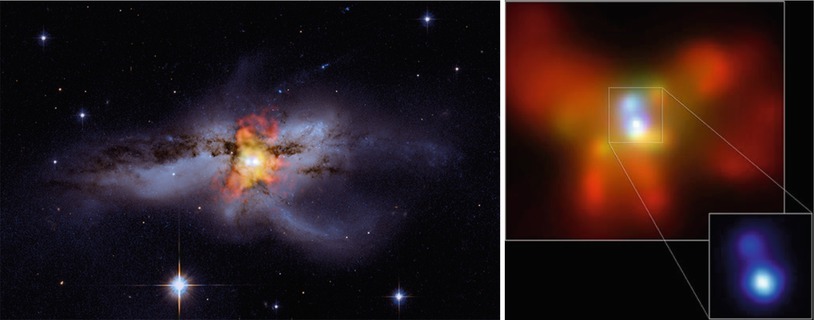
Fig. 10.19
On the
left, a composite image of the galaxy NGC 6240 (z = 0. 0245) is shown. The X-ray
emission is shown in red,
orange and yellow, superposed on an optical image
of this galaxy. A pair of two compact X-ray sources in the center,
zoomed in on the right (at
different orientation), shows the presence of two AGNs in this
galaxy; their projected separation is ∼ 1. 4 kpc. With K-band
integral field spectroscopy, the black hole mass of the more
luminous of the two AGNs has been estimated to be  .
Credit: Left: X-ray
(NASA/CXC/MIT/C. Canizares, M. Nowak); Optical (NASA/STScI).
Right: NASA/CXC/MPE/S.
Komossa et al.
.
Credit: Left: X-ray
(NASA/CXC/MIT/C. Canizares, M. Nowak); Optical (NASA/STScI).
Right: NASA/CXC/MPE/S.
Komossa et al.
.
Credit: Left: X-ray
(NASA/CXC/MIT/C. Canizares, M. Nowak); Optical (NASA/STScI).
Right: NASA/CXC/MPE/S.
Komossa et al.The galaxy NGC 6240 shown in Fig. 10.19 is a recent merger,
as seen from the disturbed morphology. Its large infrared
luminosity of  indicates that the merger induced a strong burst of star formation.
In the center of the galaxy, two AGNs are seen, revealed by their
X-ray emission. The projected separation is ∼ 1. 4 kpc in this
case.
indicates that the merger induced a strong burst of star formation.
In the center of the galaxy, two AGNs are seen, revealed by their
X-ray emission. The projected separation is ∼ 1. 4 kpc in this
case.
indicates that the merger induced a strong burst of star formation.
In the center of the galaxy, two AGNs are seen, revealed by their
X-ray emission. The projected separation is ∼ 1. 4 kpc in this
case.Several more such binary AGNs have been found,
with separation of ∼ 1 kpc or larger. In most of these systems, the
host galaxy shows signs of a recent merger, such as strongly
distorted morphology and/or intense star formation. However, one
system was found where the separation is much smaller. In the radio
galaxy 0402+379 (z = 0. 055), there are two compact
radio sources with a projected separation of 7. 3 pc, suggesting
that we are witnessing a more advanced merging stage.
Binary black holes candidates have also been
claimed from spectral studies of AGNs, where a large velocity shift
between the broad and the narrow emission lines was found. One
interpretation of these observations is that the shift is due to
the active SMBH orbiting in the host galaxy, carrying the broad
line region along its orbit, whereas the gas emitting the narrow
emission line is at rest in the host galaxy. The active SMBH can
either be a member of a binary black hole with the other one
inactive, or the merged SMBH which obtained its velocity through
recoil. AGNs with double peaked emission lines may also be
interpreted as a pair of spatially unresolved active nuclei, where
the two peaks of the emission lines reflect the line-of-sight
velocity of the two SMBHs. However, there are alternative
explanations for the nature of these sources, and the evidence for
a binary black hole is not unchallenged.
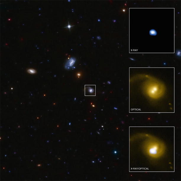
Fig. 10.20
The big multi-color optical image shows a 1
′ × 1
′ part of the
COSMOS field. The galaxy at the center is CID-42 (at z = 0. 36), of which three zoomed
images are shown on the right, with a side length of 3.
′ ′ 7. The tidal
tail seen in the optical suggests that this galaxy underwent a
merger in the more recent past. The optical images displays two
bright compact sources; only one of them has an X-ray counterpart.
Credit: X-ray: NASA/CXC/SAO/F. Civano et al; Optical:
NASA/STScI; Optical (wide field): CFHT, NASA/STScI
The galaxy CID-42 (Fig. 10.20) has two bright
optical nuclei; one of them is point-like and appears as an AGN,
whereas the other is slightly extended and most likely is a nuclear
star cluster. The AGN is also seen in X-rays, whereas the other
compact optical source has no detectable X-ray emission. The AGN is
off-center; in addition, it has broad emission lines which have a
velocity offset from the narrow emission lines of ∼ 1300 km∕s; note
that this velocity is much larger than the orbital velocity of a
binary black hole at the separation between these two compact
source components. Thus, in this system one has both kinematical as
well as positional indications for a SMBH which has been ejected
from the center of the galaxy through recoil; it is the best
candidate observed so far for this effect.
Another class of sources may indicate the
occurrence of binary SMBH mergers, the so-called X-shaped radio
sources (see Fig. 10.21). These sources are characterized by
their radio morphology, containing two pairs of jets in different
directions. The more luminous, inner pair of jets is connected to
the central source, whereas the outer jets with lower brightness
appears to consist of plasma that was ejected from the core some
time in the past. One likely possibility to explain these sources
is a change of orientation of the accretion disk, which may be due
to a change of the black hole angular momentum vector. During the
hardening of the black hole binary, the interaction of the black
holes with the gas inside the host galaxy may cause such spin
flips.
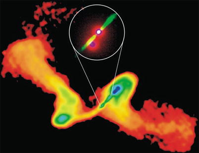
Fig. 10.21
The X-shaped radio galaxy 3C326, observed
with the VLA. The inset
shows an optical HST image of the innermost jets. The pair of radio
jets at different directions may have its origin by a change of the
black hole’s spin direction, as may occur in the process of binary
black hole mergers. Credit: Image courtesy of NRAO/AUI and Inset:
STScI
An accreting SMBH in orbit around the center of
the host galaxy can produce periodicity in its emission. The best
example yet found is the blazar OJ 287 at z = 0. 306. Variability of this object
has been traced back to 1890, using archived photographic plates,
and it shows a periodicity of 11. 86 yr. Merger models of the
source that explain the periodicity involve a second SMBH with
about 10 times lower mass. If the period of variability is
identified with the orbital period, then this binary will merge
over the next ∼ 105 yr. However, the periodicity can
have a different origin, like a precessing accretion disk, in which
case the variability could be due to changes of the jet
direction.
Overall, there are quite a number of
observational indications for binary black holes and merger
candidates. However, the best way to track down the SMBH merger
will be by observing the gravitational wave emission. The planned
space-based gravitational wave observatory LISA is expected to
detect virtually all such supermassive black hole mergers
throughout the visible Universe, and thus provide exquisite
demographics of the cosmic merger history.
10.5.3 Environmental effects on galaxy properties
Major merger events between galaxies change the
morphology and physical properties of galaxies dramatically. We
have seen that this is the probable road to the formation of normal
elliptical galaxies. However, this is not the only process in which
the properties of a galaxy can be altered; it is merely the
strongest one. Merging preferentially occurs in groups, which
combine an environment of a high number density of galaxies with a
relatively small velocity dispersion needed for mergers.
Harassment.
In clusters of galaxies, the characteristic collision speed between
galaxies is considerably higher than their internal velocity
dispersion; as we argued before, in such a case no merging can take
place. However, a high-speed collision between galaxies affect
their internal properties in a different way. If we consider such a
collision in the rest frame of one of the galaxies, then its
components experience a rapid change of the gravitational potential
as the other galaxies fly by. As a consequence, the matter in the
galaxy increases its internal energy—it is impulsively heated. This
causes the matter in the galaxy to expand, i.e., it is less
gravitationally bound than before, and therefore is more easily
affected by tidal gravitational forces. Furthermore, the heating of
the stellar component changes the distribution function (i.e., the
phase-space density f
discussed in Sect. 2.3.1) of the stars—dynamically
cold stellar disks are heated and may get destroyed, with the stars
evolving into a spheroidal distribution. The cumulative effect of
such high-speed collisions is often called galaxy harassment.
Ram-pressure
stripping and strangulation. As a galaxy orbits in a
cluster, it moves relative to the hot intracluster medium. In the
rest frame of a galaxy, the ICM acts like a wind, with the wind
speed equal to the orbital velocity of the galaxy. This wind causes
a pressure force on the interstellar medium of the galaxy; it is
proportional to the density of the ICM and the square of the
velocity. If this force is stronger than the gravitational force of
the galaxy which hosts the interstellar gas, this gas can be
removed from the galaxy. This ram-pressure stripping can thus over
time turn a gas-rich disk galaxy into a disk galaxy without gas,
i.e., a spiral galaxy into an S0 galaxy. This effect may be the
origin of the larger abundance of S0 galaxies in clusters than in
the field population. It also provides a natural explanation for
the Butcher–Oemler effect (see Sect. 6.8), which states that clusters of
galaxies at higher redshift contain a larger fraction of blue
galaxies. The blue (spiral) galaxies that have existed at higher
redshift may have turned into S0 galaxies in the meantime. The fact
that the fraction of ellipticals in a cluster remains rather
constant as a function of redshift, whereas the abundance of S0
galaxies increases with decreasing z, indicates the importance of the
latter process as an explanation of the Butcher–Oemler
effect.
Gas which is removed from the galaxies is
chemically enriched. The metallicity of the ICM is believed to be
due to the mixing of this enriched gas with the intracluster
medium. Hence, the metals of the ICM have been generated by earlier
stellar populations in cluster galaxies.
The efficiency of this effect, as well as that of
harassment, depends on the orbit of the galaxy. If the orbit comes
close to the inner part of the cluster where the gas and galaxy
number density are large, all the gas may be removed, whereas
otherwise, only the outer, more loosely bound gas is lost. In this
case, the galaxy retains its gas in the inner part and may continue
to form stars for a while; only when this gas supply is exhausted,
it then turns into a red galaxy, since no new gas can be gained
from cooling or accretion. This effect is called
strangulation.
Cannibalism. The orbit of a galaxy in a
cluster is affected by dynamical friction (see Sect. 6.3.3); it loses energy and angular
momentum, and so its orbit will shrink in time. The efficiency of
this effect again depends on the galaxy orbit; the closer it comes
to the inner parts of the cluster, the stronger are the
gravitational friction forces. Furthermore, as seen from
(6.30), it depends on the galaxy
mass, with more massive galaxies being affected more strongly.
Depending on the orbital parameters, a cluster galaxy can lose most
of its angular momentum in a Hubble time, sink to the center, and
there merge with the central galaxy. By this process, the central
galaxy becomes more massive, as it ‘cannibalized’ other cluster
members. The aforementioned mass dependence may lead to an increase
of the mass and luminosity difference between the brightest cluster
galaxy and the second-brightest one.
10.6 Evolution of the galaxy population: Numerical simulations
In the preceding sections, the formation of disk
and elliptical galaxies were described; it is generally believed
that the collapse of gas, together with its angular momentum, leads
to the formation of disk galaxies, whereas mergers and interactions
are the prime cause for the occurrence of early-type galaxies. Our
understanding of these formation processes can now in principle be
used to predict the evolution of the galaxy population in the cold
dark matter universe. The cosmological model predicts the abundance
of halos as a function of mass and redshift, the distribution of
their spin parameter, as well as the frequency of major and minor
mergers. One thus might expect that from these ingredients, the
galaxy population can well be predicted.
However, there are some major difficulties which
hamper easy progress in this direction. The evolution of galaxies
(in contrast to their dark matter halos) is strongly governed by
baryonic processes, many of which are not fully understood. For
example, we have no quantitative understanding about star
formation. The way how the explosion of a supernova feeds back
energy into the interstellar medium is subject to considerable
uncertainties; this is even more true for the feedback processes
related to AGN activity in galaxies.
A further serious problem is related to the
enormous dynamic range in length scales which are involved in
galaxy evolution in the cosmological context. We have seen that
galaxy evolution depends on the local environment; galaxies evolve
differently in groups and clusters than in the field. Hence, one
needs to consider a sufficiently large volume of the Universe such
that it contains a representative population of cluster-mass halos.
As we argued in Sect. 7.5.3, the cosmological box should
not be much smaller than 200h −1 Mpc on the side. On the
other hand, the Galactic disk has a scale-height of ∼ 100 pc, and
star formation occurs in molecular clouds with a typical size
of ∼ 1 pc. Hence, an ab initio simulation of galaxy evolution would
have to have a dynamic range of at least 108 in
length—too ambitious to be carried out.
Nevertheless, enormous progress in our
understanding of the galaxy population has been achieved in recent
years. Essentially, two different methods are used to overcome the
aforementioned problems: Historically the first was semi-analytic
modelling of the evolution of galaxies; we will discuss these
models in Sect. 10.7. But more recently, hydrodynamical
cosmological simulations have been employed to study the formation
and evolution of galaxies, which we describe in this section.
10.6.1 Numerical methods
The increase in computer power, as well as the
evolution of efficient numerical codes have allowed cosmological
simulations which include baryonic physics: heating and cooling of
gas, hydrodynamical effects etc. Simulating these processes is much
more difficult and time consuming than pure N-body simulations
which solely contain gravity—correspondingly, either their box size
and/or their spatial (and mass) resolution are smaller.
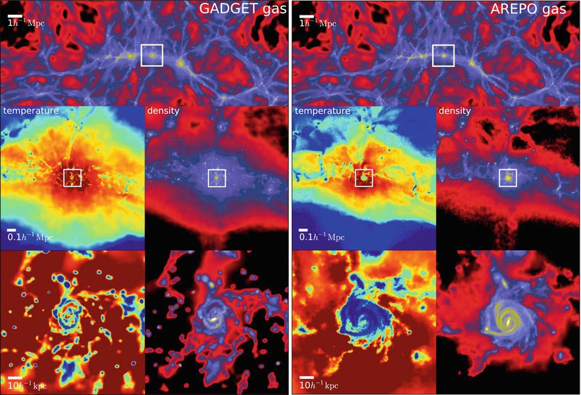
Fig. 10.22
The projected gas density from two
hydrodynamical simulations of a galaxy. Both simulations use the
same initial conditions, as well as the same prescriptions for star
formation and feedback; the only difference is the numerical method
with which the equations of hydrodynamics are treated. In the
left panel, a smooth
particle hydrodynamics (SPH) scheme was used, whereas in the
right panel the new AREPO
method was employed. The upper
panels show the gas density at redshift z = 2 in a large fraction of the full
numerical box, whereas the smaller
panels show subsequent zooms (indicated by a white square in the previous step) of
the gas temperature and density, centered on a disk galaxy. This
galaxy has significantly different properties in both simulations.
Whereas AREPO yields an extended disk with spiral arms and a bar,
the corresponding galaxy is much smaller in the SPH simulation.
Differences in the clumpiness of the medium are also visible.
Source: M. Vogelsberger et al. 2012, Moving mesh cosmology: numerical techniques
and global statistics, MNRAS 425, 3024, p. 3031, Fig. 1.
Reproduced by permission of Oxford University Press on behalf of
the Royal Astronomical Society
There are two widely spread methods for the
numerical treatment of hydrodynamics. In the first case, a
stationary grid is set up, and the differential equations of
hydrodynamics (such as the continuity and Euler equations) are
discretized on the grid.8 In the second case, the fluid is
represented by fluid particles, which are considered representative
of a mass element of gas. The interaction between these fluid
particles are prescribed such that the transport of mass, momentum,
and energy follows the laws contained in the equations of
hydrodynamics; this approach is termed smooth particle hydrodynamics (SPH) .
Different variations of these two basic schemes have been
developed. For example, in the grid-based approach, one wants to
have a higher spatial resolution in regions of large gas density;
for this purpose, one can generate sub-grids with a smaller mesh
size which yield higher spatial resolution. Such a numerical scheme
is called adaptive mesh
refinement (AMR). Lately, a new method has been developed,
which is also based on a grid; however, the grid is not stationary
but moves with the fluid, and the density of grid points adapts to
the fluid density. First tests indicate that this new scheme
(called AREPO) overcomes some of the problems of the two former
schemes and yields considerably more reliable results (see
Fig. 10.22).
The necessity for
sub-grid physics. In order to overcome the resolution
issues, several small-scale physical effects can be treated only
approximately. Since these simulations are several orders of
magnitude away from being able to resolve the formation of
molecular clouds, one needs a recipe for star formation. For
example, if the gas density exceeds a threshold value in one region
(or for one SPH particle), one assumes that a fraction of this gas
is turned into stars. In the simulation one keeps track of this
newly formed stellar population, i.e., its mass, formation time and
metallicity.
Since massive stars very quickly after formation
explode as core-collapse supernovae, for each massive star formed
(given by the total newly formed stellar mass and the assumed
initial mass function) an energy of ∼ 1051 erg is
transferred back to the surrounding gas distribution. Also this
feedback process occurs on scales below the numerical resolution,
so it is assumed that this energy is used to heat the local gas.
Also refinements have been successfully implemented, where each gas
cell or particle is split into a hot, diffuse part and a cold and
dense part. Gas can be exchanged between these two phases due to
heating and cooling processes. It turns out that the outcome of
simulations depend on the detailed prescription of this feedback
mechanism. If it is assumed that the supernova energy is
transferred mainly to the cold and dense gas, then it can be
radiated away rather quickly without affecting the dynamics of the
gas appreciably. On the other hand, if the feedback energy heats
the diffuse gas, radiative cooling is much less efficient, the gas
increases its pressure and expands, driving gas out of the dense
region (or, in physical terms, out of the disk where star formation
is located).

Fig. 10.23
Results from the Aquila Comparison Project,
in which, starting from the same initial conditions, the evolution
of a disk galaxy was followed with 13 different simulations. The
halo mass of the galaxy is similar to the one of the Milky Way,
 . The left-hand panel shows the rotation
curves of the galaxy as obtained by the different simulations, with
the rotation curve of the Milky Way shown in light grey for comparison. The
solid black curve in each
of the four subpanels is the rotation curve as obtained from a dark
matter-only simulation of the same initial conditions. In most
cases, the rotation curve has a peak at low radius, after which is
strongly declines outwards—in contrast to observed rotation curves
of spiral galaxies which are almost flat. The reason for this
behavior is the too effective cooling of gas, yielding a far too
concentrated baryonic distribution in the inner part of the galaxy.
The right panel shows, for
each of the 13 simulations, the total stellar mass as a function of
the halo mass M
200, as the galaxy evolved from redshift z = 2 (beginning of the curve) to today
(symbol). The predicted
stellar mass varies by about a factor 10 between the simulations.
The dotted curve shows the
expected stellar-to-dark matter relation, as expected from matching
the abundance of dark matter halos to that of the observed galaxy
abundance [essentially by defining a function M ∗(M 200) which brings the two
curves in Fig. 10.2 into agreement], the dashed curve shows the maximally
possible stellar mass, given by the halo mass times the mean cosmic
ratio of baryons to total matter. The two black curves (and stars) show the model predictions of
two semi-analytic models of the same halo. Source: C. Scannapieco
et al. 2012, The Aquila
comparison project: the effects of feedback and numerical methods
on simulations of galaxy formation, MNRAS 423, 1726,
p. 1734, 1735, Figs. 5, 6. Reproduced by permission of Oxford
University Press on behalf of the Royal Astronomical Society
. The left-hand panel shows the rotation
curves of the galaxy as obtained by the different simulations, with
the rotation curve of the Milky Way shown in light grey for comparison. The
solid black curve in each
of the four subpanels is the rotation curve as obtained from a dark
matter-only simulation of the same initial conditions. In most
cases, the rotation curve has a peak at low radius, after which is
strongly declines outwards—in contrast to observed rotation curves
of spiral galaxies which are almost flat. The reason for this
behavior is the too effective cooling of gas, yielding a far too
concentrated baryonic distribution in the inner part of the galaxy.
The right panel shows, for
each of the 13 simulations, the total stellar mass as a function of
the halo mass M
200, as the galaxy evolved from redshift z = 2 (beginning of the curve) to today
(symbol). The predicted
stellar mass varies by about a factor 10 between the simulations.
The dotted curve shows the
expected stellar-to-dark matter relation, as expected from matching
the abundance of dark matter halos to that of the observed galaxy
abundance [essentially by defining a function M ∗(M 200) which brings the two
curves in Fig. 10.2 into agreement], the dashed curve shows the maximally
possible stellar mass, given by the halo mass times the mean cosmic
ratio of baryons to total matter. The two black curves (and stars) show the model predictions of
two semi-analytic models of the same halo. Source: C. Scannapieco
et al. 2012, The Aquila
comparison project: the effects of feedback and numerical methods
on simulations of galaxy formation, MNRAS 423, 1726,
p. 1734, 1735, Figs. 5, 6. Reproduced by permission of Oxford
University Press on behalf of the Royal Astronomical SocietySimilarly, the accretion of gas onto a central
supermassive black hole and the corresponding feedback can be
treated only approximately. The accretion disk (or more generally,
the accretion region) can not be resolved, but the accretion rate,
and the corresponding energy output, depends mainly on the rate at
which gas can be driven into the central region of the galaxy. The
accretion rate can then be estimated from the physical conditions
on scales much larger than the accretion disk size, and is often
approximated by the Bondy–Hoyle rate [see (5.16)], bounded above by the
Eddington rate or a small multiple of it. The resulting luminosity
of the supermassive black hole is assumed to be a fraction
ε of the rest-mass energy
rate accreted, i.e.,  , with ε ∼ 0. 1 (see Sect. 5.3.5). Some fraction of this
energy output is assumed to be fed back into the surrounding gas.
This gas, being suddenly heated, will greatly expand and drive a
shock wave, by which it is blown out of the central region. This
expanding blast wave can then be followed by the hydrodynamic
solver.
, with ε ∼ 0. 1 (see Sect. 5.3.5). Some fraction of this
energy output is assumed to be fed back into the surrounding gas.
This gas, being suddenly heated, will greatly expand and drive a
shock wave, by which it is blown out of the central region. This
expanding blast wave can then be followed by the hydrodynamic
solver.The gravitational force is calculated in a very
similar way as done for pure N-body simulations, except that the
source of gravity is the sum of the densities of dark matter, gas,
stars and the central black holes. Changes to the dark matter
profile of halos due to the contraction of cooling gas is thus
included in such simulations.
Comparison of
numerical methods. We have reported some results of such
simulations above, namely simulations of the merging of two disk
galaxies (see Sect. 10.5.1). At present, the results from such
simulations need to be analyzed with care; there are still
considerable uncertainties regarding the small-scale physics (star
formation and feedback), as well as the accuracy with which the
hydrodynamical behavior of the gas can be followed. In the recent
Aquila Comparison Project, a comparison of 13 different
hydrodynamical simulations of one galaxy (where all simulations
used the same initial conditions) was performed and significant
differences were found. For example, the morphology of the galaxies
shows strong variations between the different simulations. This can
be traced back to the star-formation history: the earlier most of
the stars are formed, the less pronounced is the disk today.
Obviously, the amount of star formation in the early history of the
galaxy depends on the amount of cooling gas and, in particular, the
efficiency of feedback processes. The tendency of turning too much
gas into stars is often called the ‘overcooling problem’ in galaxy
evolution. On the other hand, the feedback must not prevent the
later accretion of gas, to build up the disk at lower
redshift.
The left hand panel of Fig. 10.23 shows the predicted
rotation curves of the galaxy, as obtained from these 13
simulations. Most of them exhibit a pronounced peak at small radii,
after which they decline outwards. Again, this is due to the
concentration of stars in the inner part of the galaxy, which not
only acts as a source of gravity by itself, but the corresponding
efficient cooling of baryons led to the contraction of the dark
matter halo. Only simulations with a very strong feedback lead to
approximately flat rotation curves; unfortunately, these models
usually do not have a well-developed disk. The compactness of the
baryonic distribution yields corresponding circular velocities
which are well above the observed Tully–Fisher relation for
spirals. The stellar mass as predicted by the models in shown in
the right-hand panel of Fig. 10.23; also here the variations between the
simulations are large, again mainly due to the different feedback
prescriptions. In some simulations, nearly all available baryons
inside the halo were turned into stars, whereas other simulations
have ∼ 10 times lower stellar mass.
Lessons. We
present this comparison here for a number of reasons. First, this
exercise shows which of the various differences between codes
matter most for the predictions and thus gives insight on how the
assumptions must be modified in order to obtain results closer to
the observed properties of galaxies. That may seem like cheating at
first sight: one turns the knobs in such a way that the results are
in agreement with observations—what about the predictive power of
such simulations then? However, one must keep in mind that some of
the key processes (to repeat: star formation and feedback) cannot
be followed from first principles, but are included in the form of
recipes. In a sense, we parametrize our ignorance, and try to
calibrate the set of parameters with a small number of key
observational facts (such as the normalization of the Tully–Fisher
relation, or the luminosity function of galaxies). The number of
different predictions from such simulations is much larger than the
number of parameters chosen; thus, once appropriate prescriptions
for the ‘sub-grid’ physics are found, these models have predictive
power.
A second, very important reason for this
discussion here is to caution the reader about the reliability of
some predictions of our cosmological model. We first note that a
similar comparison was carried out for N-body simulations, with a
very satisfactory overall agreement on scales larger than the
resolution limit (of course, on scales below the numerical
resolution, the results are even expected to be different). Thus,
the predictions concerning dark matter-only are very robust.
However, the inclusion of baryons, and the complex physical
processes they are subject to, render predictions much less
reliable. The smaller the scales and the denser the baryons, the
more non-linear are the physical processes, and the harder it is to
reliably trace them. In particular, processes on small scales have
a strong effect on large scale—e.g., feedback.
This must be taken into account when arguments
are made concerning the incompatibility of some observational
results with ΛCDM. In most
cases, these arguments concern the smallest scales or the least
massive objects, for example properties of dwarf galaxies. From
what was just stated, it is clear that currently we are not able to
make detailed predictions about observational properties of small
galaxies – when we cannot even predict the stellar mass of a
massive galaxy halo to within a factor of 3! The fact that current
simulations fail to reproduce spirals which fit the Tully–Fisher
relation is most likely not a failure of the underlying
cosmological model, but a lack of understanding of the complex
small-scale physical processes involved.9
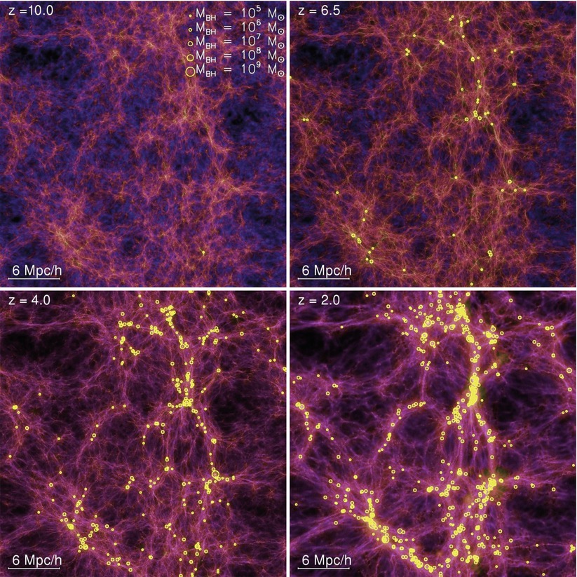
Fig. 10.24
The density of baryons from a
hydrodynamical simulation, projected over a 5h −1 Mpc thick slice.
Intensity and color indicate gas surface density and
temperature, respectively. Four snapshots at different redshifts
are shown. Yellow circles
indicate the location of supermassive black holes, with the
symbol size indicating the
black hole mass. In this simulation, for which a box of size
 was chosen, it was
assumed that 5 % of the AGN luminosity is fed back to the
interstellar medium; this choice was made in order to reproduce the
observed relation between black hole mass and velocity dispersion
of the spheroidal stellar component. Source: T. di Matteo
et al. 2008, Direct
Cosmological Simulations of the Growth of Black Holes and
Galaxies, ApJ 676, 33, p. 38, Fig. 1. ©AAS. Reproduced with
permission
was chosen, it was
assumed that 5 % of the AGN luminosity is fed back to the
interstellar medium; this choice was made in order to reproduce the
observed relation between black hole mass and velocity dispersion
of the spheroidal stellar component. Source: T. di Matteo
et al. 2008, Direct
Cosmological Simulations of the Growth of Black Holes and
Galaxies, ApJ 676, 33, p. 38, Fig. 1. ©AAS. Reproduced with
permission10.6.2 Results
The challenge for models of galaxy evolution is
to explain the observational results of the galaxy population at
low and high redshift. In this section, we will illustrate the
current status of gas-dynamical cosmological simulations and their
ability to reproduce key observations.
Growth of black
holes and galaxies. The tight correlation between central
black hole mass and properties of the spheroidal stellar component
in galaxies suggest a close connection of the evolution of both
components. Furthermore, feedback processes from AGN activity are
essential for understanding the evolution of galaxies. We next
present some results of a gas-dynamical cosmological simulation
which includes the evolution of the supermassive black holes in
galactic centers. For this simulation, the Bondi–Hoyle accretion
rate was assumed, as described above. All halos, once they exceed a
mass threshold, were artificially provided with a seed black hole
of  at the location of the densest gas
particle, thereby circumventing our lack of understanding on how
the first massive black holes were formed. The mass of the seed
black hole is rather unimportant as long as it is much smaller than
the mass at later times. In particular, the total mass in these
seed black holes is a minute fraction of the total mass of black
holes at later epochs which is totally dominated by accretion
processes.
at the location of the densest gas
particle, thereby circumventing our lack of understanding on how
the first massive black holes were formed. The mass of the seed
black hole is rather unimportant as long as it is much smaller than
the mass at later times. In particular, the total mass in these
seed black holes is a minute fraction of the total mass of black
holes at later epochs which is totally dominated by accretion
processes.Figure 10.24 shows the gas density and temperature in
the simulation box, together with the location of black holes. As
expected, these are located in the center of density maxima. The
black hole distribution traces the overall density distribution,
although with considerable scatter. The number density of black
holes varies strongly between filaments of gas which apparently
have very similar density. Already at redshift z = 6. 5, quite a number of black holes
have formed, some with masses close to  , although no SMBH has formed with
masses needed to explain the luminous quasars seen at
, although no SMBH has formed with
masses needed to explain the luminous quasars seen at  (i.e.,
  ). However,
these quasars have a very low space density, and one cannot expect
to find such massive black holes in a simulation box of the size
considered here.
). However,
these quasars have a very low space density, and one cannot expect
to find such massive black holes in a simulation box of the size
considered here.
, although no SMBH has formed with
masses needed to explain the luminous quasars seen at
(i.e., ). However,
these quasars have a very low space density, and one cannot expect
to find such massive black holes in a simulation box of the size
considered here.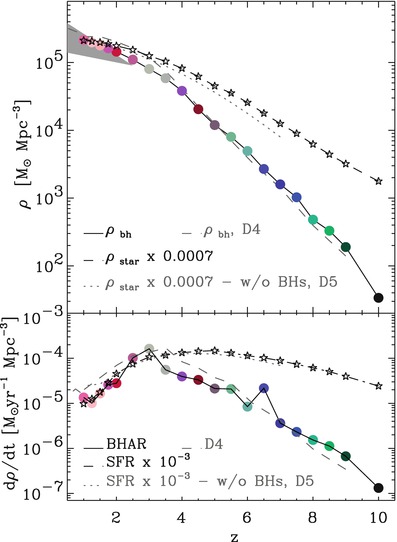
Fig. 10.25
The upper
panel shows the mass density of black holes as a function of
redshift (colored points
and solid curve), for the
simulation shown in Fig. 10.24. The lower dashed curve shows the same
quantity for a simulation with the same initial conditions and
physical assumptions, but lower mass resolution, indicating that
this prediction of the model is not strongly affected by resolution
effects. The dashed curve
and the star symbols show
the mean density of stars, scaled by a factor 7 × 10⁻⁴,
whereas the dotted curve
shows the stellar mass density from the same simulation, but where
the feedback from the accreting black holes was absent. The
shaded grey triangle at low
redshifts shows estimates of the black hole mass density from
observations. The lower
panel displays the growth rate of the black hole mass
density and stellar mass density, with the same line styles as in
the upper panel. Source: T. di Matteo et al. 2008,
Direct Cosmological Simulations of
the Growth of Black Holes and Galaxies, ApJ 676, 33, p. 41,
Fig. 4. ©AAS. Reproduced with permission
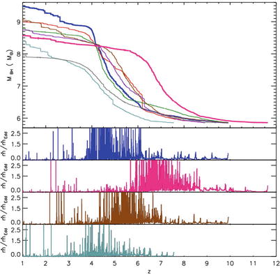
Fig. 10.26
The upper
panel shows the mass of the six most massive black holes at
z = 1, as well as that of
two intermediate mass black holes, as a function of redshift. The
two thicker lines highlight
the most massive SMBHs in this simulation at z = 6 and at z = 1. The lower panels display the accretion rate
in units of the Eddington rate as a function of redshift, with the
same color coding as in the upper panel. Source: T. di Matteo
et al. 2008, Direct
Cosmological Simulations of the Growth of Black Holes and
Galaxies, ApJ 676, 33, p. 48, Fig. 13. ©AAS. Reproduced with
permission
The total mass density of the SMBHs in the
simulation as a function of redshift is shown in the upper panel of
Fig. 10.25
where it is compared to the mean mass density of stars. We see that
the SMBH density increases faster with cosmic time than the stellar
mass density, which shows that the evolution of the stellar density
precedes that of the SMBH. This is shown more clearly in the lower
panel, where the growth rate of these densities are displayed
(i.e., the time derivative of the curves in the upper left panel).
Both growth rates exhibit a peak at intermediate redshifts;
however, whereas the peak in the stellar mass density is fairly
broad (as observed in the Madau diagram—see Fig. 9.55), it is much more peaked for
the black holes. Comparing the mass density of the SMBH population
with observational estimates, one finds broad agreement.
It is instructive to consider the mass history of
individual black holes in the simulation, which is displayed in the
upper panel of Fig. 10.26 for the six most massive (at z = 1) black holes and two less massive
ones. The growth of the SMBH mass is quite rapid at the beginning,
and apparently episodic. The mass accretion rate in units of the
Eddington rate (5.27) for four of the SMBHs is
plotted in the lower panels (note that for this simulation, the
maximum accretion rate was chosen to be three times the Eddington
rate). The most massive black holes undergo extended periods where
the accretion rate is very high, limited only by the Eddington
ratio. Hence, these holes grow as fast as possible in these
periods, since there is enough supply of fuel—presumably in the
aftermath of a major merger. The most massive SMBH at z = 6 (pink curves) undergoes a very
extended period of accretion between redshifts 5 and 7, after which
it turns to become very inactive, with the exception of a few short
episodes of accretion during which its mass is only slightly
increased. The blue curve shows the most massive SMBH at
z = 1, which started
massive accretion only at redshift z ≲ 6, but then rapidly grew in mass.
Hence we infer from the figure that the fates of individual SMBHs,
and their corresponding AGN activity, are quite diverse.
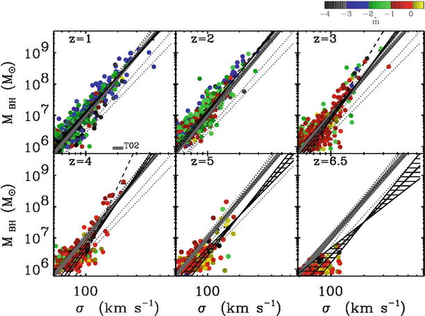
Fig. 10.27
From the same simulations as in
Fig. 10.24,
the black hole mass is plotted as a function of the velocity
dispersion σ of the stellar
mass particles within the half-mass radius, for six different
redshifts as indicated. The thick
grey line in all panels is the best fit to the local
M •-σ relation. For each redshift, a
power-law relation was fitted to the points, which is shown as
solid line, together with
its 1-σ uncertainty (as
hatched region; for the low redshifts, this uncertainty is so small
that the hatched region is essentially invisible). The dotted lines in each panel show the
power-law fits obtained at the other redshifts, increasing from top
to bottom. The color of
each point codes the accretion rate of the SMBH at the snapshot, in
units of the Eddington accretion rate, with the corresponding color
bar at the top of the figure. Source: T. di Matteo et al.
2008, Direct Cosmological
Simulations of the Growth of Black Holes and Galaxies, ApJ
676, 33, p. 44, Fig. 8. ©AAS. Reproduced with permission
One of the most promising results of the
simulation is the strong correlation between black hole mass and
the velocity dispersion of the stellar component, as shown for six
different redshifts in Fig. 10.27. There we see that beginning with
z ∼ 4, the best-fit
relation from the simulation agrees with the locally observed one
(see Fig. 3.45). The normalization of the
power-law fits depends on the assumed fraction of AGN luminosity
that is available for feedback, chosen to be 5 % here. However,
more exciting than the precise normalization of this relation is
the fact that hierarchical galaxy evolution is able to explain the
observed tight correlation without additional ad-hoc assumptions.
Also seen is that the tight relation is satisfied by black holes
independent of their accretion state—i.e., active and inactive SMBH
lie on the same relation.
However, it must be pointed out that the
resolution of these simulations do not allow statements about the
morphology of galaxies; therefore, the velocity dispersion plotted
in Fig. 10.27
is that of the total stellar population, not that of the spheroidal
component only, for which the M •-σ relation is observed.
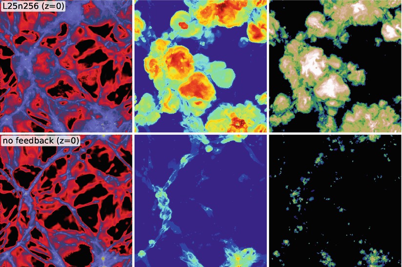
Fig. 10.28
Gas-dynamical simulations of structure
formation, with (top) and
without (bottom) the
inclusion of feedback processes. Shown is the distribution of gas
density (left), temperature
(middle) and metallicity
(right) at z = 0, over an area 25h −1Mpc on the side and
projected over a slab of thickness 1h −1Mpc. Source: M.
Vogelsberger et al. 2013, A
model for cosmological simulations of galaxy formation
physics, arXiv:1305.2913, Fig. 3. Reproduced by permission
of the author
Impact of feedback
on the gas. The foregoing discussion has shown the
challenges of hydrodynamic cosmological simulations, in particular
concerning numerical resolution and the implementation of sub-grid
physics. We present next some recent results from simulations
carried out with the AREPO code (see Fig. 10.22). Several runs were
produced in which the parameters of the description for sub-grid
physics were varied. The properties of the feedback by supernovae,
which result in an outflow (‘wind’), were varied, both concerning
the mass rate of the outflow as well as its velocity. Furthermore,
several feedback descriptions of AGNs were employed.
Figure 10.28 illustrates the importance of the
feedback on the properties of the gas. As seen in the left-hand
panels, the distribution of the gas density is more extended when
feedback processes are included, as the outflows generated by
supernovae and AGN feedback distributes the gas over a larger
volume, whereas in a model with no feedback, the high-density gas
is more confined to dark matter halos and the denser regions of the
dark matter filaments. The impact of feedback is more dramatic on
the distribution of gas temperature, as seen in the middle panels;
without feedback, hot gas is confined to the densest regions,
whereas the action of strong radio-mode AGN activity distributes
hot gas over large regions of space. The feedback-driven outflows
also lead to a wide-spread enrichment of the intergalactic gas with
metals (right-hand panels), which otherwise would stay close to
their source of origin, i.e., the inner regions of halos in which
stellar evolution takes place, in sharp contrast to observations of
QSO absorption which show that the IGM is metal enriched.
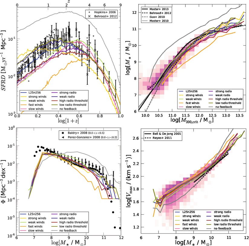
Fig. 10.29
Several results from the hydrodynamical
simulations shown in Fig. 10.28 are displayed here. In all cases, the
blue curve shows the
simulation where all the free parameters of the model were set to
their fiducial values. The other curves show variations of this model,
which differ from the fiducial model by changing the prescription
of various feedback processes by supernovae (these relate to the
strong/weak/fast/slow wind models) and AGN. The grey curve corresponds to a model with
no feedback. Top left: The
star formation rate density as a function of redshift (i.e., the
‘Madau plot’). Black
symbols with error bars show estimates from observations, as
described in Sect. 9.6.2, whereas the curves show the results from the
simulation. Top right: The
stellar mass vs. halo mass. The shading indicates the probability
density for the fiducial model, with the blue curve showing the median of
M ∗ at fixed
halo mass. The black curves
show estimates of the M
∗(M
200)-relation as obtained from abundance matching of
galaxies with dark matter halos, the other curves correspond to variants of the
numerical model. Bottom
left: The stellar mass function at z = 0, compared to observational
results (symbols with error bars). Bottom right: The maximum rotational
velocity V max
of galaxies as a function of their stellar mass, i.e., the
Tully–Fisher relation, for z = 0. The shading shows the probability density
for the fiducial model, with the blue curve showing the median of
V max at fixed
M ∗. The two
black lines show the
observed Tully–Fisher relation, the other curves variations of the
fiducial model. Source: M. Vogelsberger et al. 2013,
A model for cosmological
simulations of galaxy formation physics, arXiv:1305.2913,
Figs. 6, 7, 8, 10. Reproduced by permission of the author
The star-formation
rate density. Every successful model of galaxy evolution
must be able to reproduce the observed star-formation history in
the Universe. We have seen in Sect. 9.6.2 that the star-formation rate
density evolves strongly with redshift, showing a broad peak at
redshifts between 2 and 4. The top left panel of Fig. 10.29 shows a recent
version of the Madau-diagram, and predictions from the numerical
simulations. Here and in the other panels of the figure, the blue
curve corresponds to the fiducial set of feedback parameters, and
the other colored curves show variations of the model. Whereas the
fiducial model provides a satisfactory fit to the observational
results, some of the other models fail dramatically. Foremost, the
model with no feedback overproduces stars by a large factor, and
can safely be ruled out also for this reason. Changing the feedback
from SNe can also alter the model prediction substantially; for
example, the model termed ‘fast winds’ blows the gas out of halos
and thus prevents the formation of stars at later epochs. Strong
winds remove the gas from halos at early times, thus reducing the
star-formation rate, but later gas is reaccreted and results in
star formation rates at low redshifts which are larger than those
estimated from observations. Other parameter variations are seen to
have a smaller impact on the predictions.
The stellar
mass-halo mass relation. We saw in Sect. 7.7.4 that the ratio of
M ∗∕M 200 varies substantially
with M 200,
which is the origin for the mismatch between the halo mass function
and the stellar mass function, shown in Fig. 10.2. In particular, this
ratio attains a maximum at a characteristic mass scale which
corresponds to a massive galaxy in the current Universe. The top
right panel of Fig. 10.29 shows the predictions of the  -relation from the simulations,
compared to the observed relation (shown as black curves). The
fiducial model appears to reproduce the observed relation quite
well, though the turnover at
-relation from the simulations,
compared to the observed relation (shown as black curves). The
fiducial model appears to reproduce the observed relation quite
well, though the turnover at  is less
pronounced than that obtained from observations. The ‘fast wind’
model fails in a similar way as for the star-formation rate
density—too much gas is blown out of halos. In general, variations
of AGN feedback affect the upper mass end of the relation more
strongly than for lower masses, and is essential for the
suppression of star formation in high-mass halos, as argued several
times before. Conversely, the low-mass end of the relation is more
sensitive to feedback from supernovae.
is less
pronounced than that obtained from observations. The ‘fast wind’
model fails in a similar way as for the star-formation rate
density—too much gas is blown out of halos. In general, variations
of AGN feedback affect the upper mass end of the relation more
strongly than for lower masses, and is essential for the
suppression of star formation in high-mass halos, as argued several
times before. Conversely, the low-mass end of the relation is more
sensitive to feedback from supernovae.
-relation from the simulations,
compared to the observed relation (shown as black curves). The
fiducial model appears to reproduce the observed relation quite
well, though the turnover at is less
pronounced than that obtained from observations. The ‘fast wind’
model fails in a similar way as for the star-formation rate
density—too much gas is blown out of halos. In general, variations
of AGN feedback affect the upper mass end of the relation more
strongly than for lower masses, and is essential for the
suppression of star formation in high-mass halos, as argued several
times before. Conversely, the low-mass end of the relation is more
sensitive to feedback from supernovae.The stellar mass
function of galaxies. Successful galaxy evolution models
should be able to reproduce the observed luminosity function of
galaxies, as a function of redshift. Since the prediction of the
luminosity in a specific spectral band depends not only on the
properties of the stellar population, but also on the dust content
and distribution, the calculated luminosity function is affected by
an additional uncertainty. For that reason, a comparison of the
stellar mass function between simulations and observations is
slightly more straightforward. This is shown in the bottom left
panel of Fig. 10.29, where the stellar mass function from the
simulations is compared to observational results at low redshifts.
The cut-off below M
∗ ∼ 107. 5 is due to the finite resolution of
the simulations which implies a minimum halo mass that can be
resolved. Models with fast or strong winds from supernovae severely
underpredict the mass function over a broad mass range. The impact
of AGN feedback is most clearly seen at and beyond the mass scale
where the mass function starts to bend over; in particular,
reducing the strength of AGN feedback overpredicts the stellar mass
function at the high-M
∗ end.
The Tully–Fisher
relation. Finally, the lower right panel of
Fig. 10.29
compares the observed Tully-Fisher relation with the model
prediction. The fiducial model reproduces the observed relation
fairly well, but the changes that occur by altering the feedback
model parameters are modest in this case. However, the model
without AGN feedback fails also this comparison, yielding a much
steeper relation than observed.
Conclusion.
The example just presented shows that modern hydrodynamic
simulations of galaxy evolution can reproduce some key observables.
By comparing the predictions from the model to observations, the
various free parameters describing the sub-grid physics can be
adjusted. Whereas the ‘fiducial model’ fares quite well in the
comparison shown, there remain several shortcomings. For example,
the observed mass-metallicity relation (see Fig. 3.40) is not well matched by the
simulation, whereas the stellar mass-black hole mass relation can
be reproduced fairly well. Without doubt, this field will see
further strong developments in the future.
10.7 Evolution of the galaxy population: Semi-analytic models
Hydrodynamic simulations are difficult and
computationally expensive. This means that one cannot carry out
large numbers of such simulations, for example, to test a large
number of different parameter sets for the sub-grid physics (like
feedback efficiency). Furthermore, their spatial resolution and/or
the total volume covered by these simulations are typically
inferior to those of pure N-body simulations. Hence, it is a larger
challenge to include both the large-scale density perturbations in
the matter field (on scales larger than ∼ L∕2), and the high resolution necessary
to resolve the smaller-mass galaxies.
Instead, one can follow a different approach, in
which the behavior of the dark matter distribution is obtained from
N-body simulations, and simplified descriptions of the behavior of
baryons in this matter distribution are employed. The formation of
galaxies happens in dark matter halos, and so each dark matter halo
is a potential site for the formation of stars—i.e., a galaxy. At
the moment a halo forms, one expects that it contains a baryon
fraction equal to the cosmic mean, and that the baryons have
approximately the same spatial distribution and the same specific
angular momentum as the dark matter (which is obtained from the
N-body simulation). The fate of the baryons then depends on various
physical processes which we have already discussed above: cooling,
star formation, supernova feedback, accretion of gas onto a central
black hole, etc. Furthermore, the N-body simulation yield the
merging history of all dark matter halos, and so the processes
which occur in minor and major mergers can be treated as
well.
Some of these processes are rather well
understood, such as cooling, whereas for those physical processes
which we are unable to describe with a quantitative physical model,
a parametrized, approximate description is chosen. To give one
example, the star-formation rate in a galactic disk is expected
(and observed) to depend on the local surface mass density
Σ g of gas in
the disk. Therefore, the star-formation rate is parametrized in the
form  [see (3.16)], and the parameters
A and β adjusted by comparison of the model
predictions with observations. Such semi-analytic models of galaxy
formation and evolution have contributed substantially to our
understanding and interpretation of observations. We will discuss
some of the properties and predictions of these models in the
following.
[see (3.16)], and the parameters
A and β adjusted by comparison of the model
predictions with observations. Such semi-analytic models of galaxy
formation and evolution have contributed substantially to our
understanding and interpretation of observations. We will discuss
some of the properties and predictions of these models in the
following.10.7.1 Method for semi-analytic modeling
Merger
trees. The distribution of particles resulting from an
N-body simulation at a given output time can be used to identify
dark matter halos. Several methods for that can be applied as
described in Sect. 7.5.3, e.g., the friends-of-friends
method, the spherical overdensity criterion, or a combination of
these. Similarly, sub-halos within each halo can be identified as
well. Comparing the lists of (sub-)halos and their particle
contents at consecutive output times, one can identify whether a
halo present at the earlier time has merged with another halo
before the later output time. Over the course of time, more and
more smaller halos have merged to more massive ones. Thus, for each
halo at redshift z = 0, one
can follow its complete merging history back in time, thereby
obtaining its ‘merger tree’ (see Fig. 10.30).10
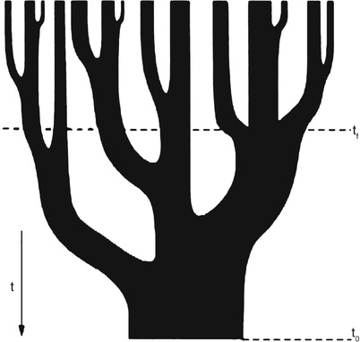
Fig. 10.30
A typical merger tree, as expected in a
hierarchical CDM model of structure formation. The time axis runs
from top to bottom. A massive halo at the present time t 0 has formed by mergers of
numerous halos of lower mass, as indicated in the figure. One
defines the time of halo formation as the time t f at which one of the
sub-halos had reached half the mass of the current halo. Source: C.
Lacey & S. Cole 1993, Merger
rates in hierarchical models of galaxy formation, MNRAS 262,
627, p. 636, Fig. 6. Reproduced by permission of Oxford University
Press on behalf of the Royal Astronomical Society
Gas cooling and
star formation. In a halo where no merger process occurs at
a given time, gas can cool. The cooling rate is determined by the
chemical composition and the density of the gas as we described
above. Besides the cooling processes, one can also account for the
heating of the gas by the ionizing background radiation.
Furthermore, one can account for the fact that low-mass halos are
expected to have a smaller baryon fraction than the cosmic mean, if
the gas is heated by the ionizing background to temperatures higher
than the virial temperature of the halo, as described by
(10.10).
Cool gas is assumed to settle down in a
rotationally-supported thin disk. If the density of the gas is
sufficiently high, it can form stars, where the star-formation rate
is assumed to follow the Schmidt–Kennicutt law (3.16), averaged over the disk. A
simpler prescription for star formation is  ,
where M cool is
the mass of cold gas in the halo, and τ a characteristic time, such as the
dynamical time-scale of the disk. The newly formed stars are
associated with a ‘disk component’.
,
where M cool is
the mass of cold gas in the halo, and τ a characteristic time, such as the
dynamical time-scale of the disk. The newly formed stars are
associated with a ‘disk component’.
,
where M cool is
the mass of cold gas in the halo, and τ a characteristic time, such as the
dynamical time-scale of the disk. The newly formed stars are
associated with a ‘disk component’.Supernova
feedback. Shortly after the formation of stars, the more
massive of them will explode in the form of supernovae. This will
re-heat the gas, since the radiation from the SN explosions and, in
particular, the kinetic energy of the expanding shell, transfers
energy to the gas. By this heating process, some of the cool gas
can be heated again and be driven out into the halo, i.e., the hot
gas mass of the halo is increased in this way. Furthermore, if the
energy input by supernova feedback is large enough, the heated gas
can actually be expelled from the halo altogether (and at some
later time reaccreted onto the halo). The suppression of the
formation of low-mass galaxies by the effects mentioned here is a
possible explanation for the apparent problem of CDM substructure
in halos of galaxies discussed in Sect. 7.8. In this model, CDM sub-halos
would be present, but they would be unable to have experienced an
efficient star-formation history—hence, they would be dark.
In any case, feedback reduces the amount of cold
gas available for star formation. This leads to a self-regulation
of star formation, which prevents all the gas in a halo from being
transformed into stars. This kind of self-regulation by the
feedback from supernovae (and, to some extent, also by the winds
from the most massive stars) is also the reason why the star
formation in our Milky Way is moderate, i.e., not all the gas in
the disk is involved in the formation of stars.
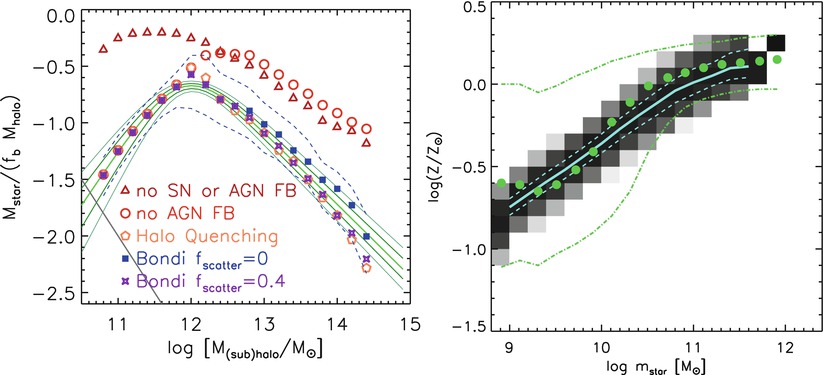
Fig. 10.31
Left
panel: The fraction of baryons in the form of stars, as a
function of halo mass, as predicted by a semi-analytic model. The
brown triangles show the
stellar mass fraction for a model run where no feedback was
included. In this case, for galaxy-mass halos ( ) most of the baryons have
been converted into stars. For larger halos masses, the fraction
decreases, since cooling becomes less efficient in these halos. The
green curves show the range
of stellar mass fractions that is obtained from observations.
Obviously, the no-feedback assumption violates observational
constraints on all mass scales. The red circles show results from a model
in which supernova feedback was included, but no feedback from AGN.
Here, the stellar mass fraction is very substantially reduced at
the low-mass end, bringing it into the observed range; however,
supernovae are inefficient at high halo masses. The other three
types of symbols correspond
to different assumptions about AGN feedback; clearly, AGN feedback
is needed to account for the small star-formation efficiency in
high-mass halos, such as groups and clusters. Right panel: The metallicity as a
function of stellar mass. Grey
shades indicate the probability distribution that a galaxy
of stellar mass m
star has a metallicity Z (in Solar units), with the
solid curve showing the
median and the dashed curve
the 1-σ range, as obtained
from a semi-analytic model. The green points show the observed
metallicity of galaxies. The median of the two distributions agree
very well, though the spread is considerably larger in the observed
galaxies. Source: R. Somerville et al. 2008, A semi-analytic model for the co-evolution of
galaxies, black holes and active galactic nuclei, MNRAS 391,
481, p. 492, 494, Figs. 3, 6. Reproduced by permission of Oxford
University Press on behalf of the Royal Astronomical Society
) most of the baryons have
been converted into stars. For larger halos masses, the fraction
decreases, since cooling becomes less efficient in these halos. The
green curves show the range
of stellar mass fractions that is obtained from observations.
Obviously, the no-feedback assumption violates observational
constraints on all mass scales. The red circles show results from a model
in which supernova feedback was included, but no feedback from AGN.
Here, the stellar mass fraction is very substantially reduced at
the low-mass end, bringing it into the observed range; however,
supernovae are inefficient at high halo masses. The other three
types of symbols correspond
to different assumptions about AGN feedback; clearly, AGN feedback
is needed to account for the small star-formation efficiency in
high-mass halos, such as groups and clusters. Right panel: The metallicity as a
function of stellar mass. Grey
shades indicate the probability distribution that a galaxy
of stellar mass m
star has a metallicity Z (in Solar units), with the
solid curve showing the
median and the dashed curve
the 1-σ range, as obtained
from a semi-analytic model. The green points show the observed
metallicity of galaxies. The median of the two distributions agree
very well, though the spread is considerably larger in the observed
galaxies. Source: R. Somerville et al. 2008, A semi-analytic model for the co-evolution of
galaxies, black holes and active galactic nuclei, MNRAS 391,
481, p. 492, 494, Figs. 3, 6. Reproduced by permission of Oxford
University Press on behalf of the Royal Astronomical SocietyThe left panel of Fig. 10.31 shows the
importance of supernova feedback. Plotted here is the stellar mass
fraction of baryons as a function of halo mass. A semi-analytic
model without the inclusion of feedback yields the result that for
halo masses below  , more than half of the
baryons are contained in stars. This is in sharp contradiction to
observations which show that star formation is a rather inefficient
process. This is just one of several arguments—in the absence of
feedback, a Milky Way-like galaxy would have consumed all its gas
early in its history, leaving no gas reservoir for current star
formation. Including supernova feedback, the stellar mass fraction
of the model can be made to agree with observations, for
galaxy-mass halos. For more massive halos, feedback by supernovae
is no longer efficient, and a different feedback mechanism is
required (see below).
, more than half of the
baryons are contained in stars. This is in sharp contradiction to
observations which show that star formation is a rather inefficient
process. This is just one of several arguments—in the absence of
feedback, a Milky Way-like galaxy would have consumed all its gas
early in its history, leaving no gas reservoir for current star
formation. Including supernova feedback, the stellar mass fraction
of the model can be made to agree with observations, for
galaxy-mass halos. For more massive halos, feedback by supernovae
is no longer efficient, and a different feedback mechanism is
required (see below).Minor
mergers. The merger trees obtained from the N-body
simulations describe for each halo at which time it merges with
another one. As we discussed above, the outcome of a merger will
depend to a large degree on the mass ratio of the two merging halos
(and galaxies): If the mass ratio is substantially different from
unity (e.g., smaller than 1:3; minor merger), the merger will cause
little damage to the galaxy of the more massive component, whereas
for almost equal mass mergers, one expects that both galaxies will
be destroyed and the stellar distribution be changed
drastically.
If the masses of the two components in a merger
are very different, the merging process of the two components does
not occur instantaneously, but since the smaller galaxy will have,
in general, a finite orbital angular momentum, it will first enter
into an orbit around the more massive component. The smaller mass
halo and galaxy can survive as a satellite galaxy. This satellite
galaxy is subject to several processes, though. By moving through
the hot gas of the larger halo, ram-pressure stripping can remove
gas, at a rate depending on the gas density in the halo, the orbit
of the satellite (as determined by the N-body simulation), and the
gas density of the satellite (which has been recorded by the
earlier evolution of that galaxy before the merger event). The
stripped gas is added to the gas distribution of the main halo. The
stripping of the gas reduced the reservoir from which the satellite
can form stars, a process which explains that satellite galaxies in
groups and clusters are usually redder than their central
galaxy.
Furthermore, dynamical friction (see
Sect. 6.3.3) changes the orbit of the
satellite in time, bringing it closer to the halo center. Once that
happens, the cold gas and the stars of the satellite galaxy are
added to the disk component of the central galaxy of the
halo.
It may also be that the orbit of a satellite
galaxy comes close to the center of the main halo where the tidal
forces are strong. In such a case, the galaxy may be tidally
disrupted. Since the satellite in this case has a large velocity
relative to the central galaxy, its stars are then assumed to be
dispersed in the halo, contributing to the intracluster stellar
population which has been found in individual clusters, as well as
in the cluster population as a whole (see Sect. 6.3.4). Since the cold gas and the
stars are more concentrated than the dark matter subhalo of the
satellite, the galaxy (i.e., stars + gas) may survive tidal
effects, even after the dark matter subhalo has been tidally
disrupted. Hence, there may be orphan galaxies—satellite galaxies
without a corresponding dark matter subhalo.
Major
mergers. If the two merging galaxies have a mass ratio close
to unity (i.e., larger than ∼ 1: 3), it is assumed that their disks
are completely destroyed and their stars being rearranged into a
spheroidal distribution. Furthermore, a fraction of the sum of the
cold gas in both components is assumed to undergo a starburst. The
newly formed stars are added to the spheroidal stellar component.
For minor mergers, a corresponding collisional starburst can be
added as well, where the newly formed stars are added to the disk
component. The resulting strong supernova feedback can then expel
most of the remaining gas from the remnant of a major merger,
leaving a (gas-poor) elliptical galaxy.
After the formation, an elliptical can attain new
cold gas from the cooling of hot gas in the halo, accretion of
surrounding material, or subsequent minor merger events. By these
processes, a new disk population may form. In this model, a spiral
galaxy is created by forming a bulge in a ‘major merger’ at early
times, with the disk of stars and gas being formed later in minor
mergers and by accretion of gas. Hence the bulge of a spiral is, in
this picture, nothing but a small elliptical galaxy, which is also
suggested by the very similar characteristics of bulges and
ellipticals, including the fact that both types of objects seem to
follow the same relation between the black hole mass and the
stellar velocity dispersion, as explained in Sect. 3.8.3.
Black hole growth,
and feedback from AGN. When they form, galaxies are
implanted a central black hole of small seed mass, as described
above for the hydrodynamical simulations. The mass of the black
holes then grows as a result of mergers and accretion of gas. The
former process drives gas into the center of the galaxies, where a
star-formation episode sets in; this process also feeds gas onto
the supermassive black hole. The two SMBHs in a merger event are
assumed to also merge. In this mode of accretion, star formation
and AGN activity happen in parallel, and so do the corresponding
feedback processes. Hence, only their sum is relevant.
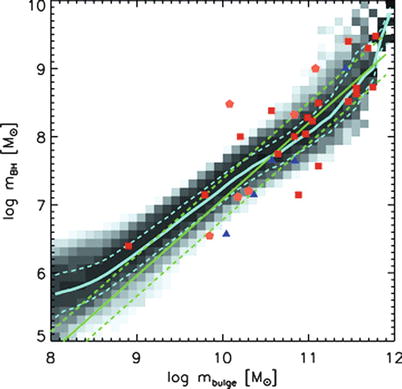
Fig. 10.32
The black hole mass vs. bulge mass
relation, as predicted from a semi-analytic model. Grey shading indicates the probability
distribution of the black hole mass for a given bulge mass, the
blue solid and dashed curves yield the median of the
black hole mass and its 1-σ
range. The green lines show
the corresponding results from observations, whereas symbols show individual observed
galaxies. Source: R. Somerville et al. 2008, A semi-analytic model for the co-evolution of
galaxies, black holes and active galactic nuclei, MNRAS 391,
481, p. 495, Figs. 7. Reproduced by permission of Oxford University
Press on behalf of the Royal Astronomical Society
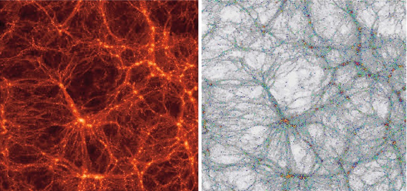
Fig. 10.33
On the
left, the distribution of dark matter resulting from an
N-body simulation is shown.
The dark matter halos identified in this mass distribution were
then modeled as the location of galaxy formation—the formation of
halos and their merger history can be followed explicitly in the
simulations. Semi-analytic models describe the processes which are
most important for the gas and the formation of stars in halos,
from which a model for the distribution of galaxies is built. In
the panel on the right, the
resulting distribution of model galaxies is represented by
colored dots, where the
color indicates the spectral energy distribution of the respective
galaxy: galaxies with active star formation are shown in
blue, while galaxies which
are presently not forming any new stars are marked in red. The latter are particularly
abundant in clusters of galaxies—in agreement with observations.
Credit: G. Kauffmann, J. Colberg, A. Diaferio & S.D.M. White,
and the GIF-Collaboration
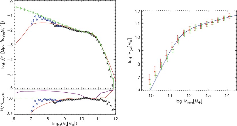
Fig. 10.34
Upper left
panel: The stellar mass function of galaxies as obtained
from a semi-analytic model for which the Millennium Simulation (MS)
and the Millennium II (MS-II) simulations have been used for
describing the dark matter evolution (see Sect. 7.5.3). The red and green curves show the model predictions
from the MS and the MS-II, respectively. Owing to the better
spatial and mass resolution of the MS-II, the stellar mass function
can be followed to considerably smaller masses. Black and blue points show observational results
as obtained from the SDSS; at the lowest mass end, the observed
galaxies come from a very small local volume, and are therefore
subject to a substantial ‘cosmic variance’. The lower left panel shows the ratio of
the mass functions relative to the predictions from the MS-II.
Clearly, the semi-analytic model can reproduce the observed mass
function accurately over some 4 orders of magnitude (the
purple curve in the lower
panel shows the corresponding results from an earlier incarnation
of semi-analytic modelling, where in particular the feedback was
assumed to be weaker). The right
panel shows the mean stellar mass and its dispersion as a
function of the halo mass, as obtained from the simulations.
Green symbols are for
central galaxies of halos, whereas the red symbols correspond to satellite
galaxies (where the corresponding halo mass is the mass of their
subhalos at the time the satellite has merged with the main halo).
The blue curve is obtained
if the dark matter halo abundance is directly matched to the
stellar mass function, assuming a monotonic dependence between
these two quantities. Note that the slope of the relation is
considerably steeper than unity at the low-mass end, and much
flatter at the high-mass end. This relation therefore explains the
different shapes of the halo mass and stellar mass functions shown
in Fig. 10.2.
Source: Q. Guo et al. 2011, From dwarf spheroidals to cD galaxies:
simulating the galaxy population in a ΛCDM cosmology, MNRAS
413, 101, p. 115, 117, Figs. 7, 9. Reproduced by permission of
Oxford University Press on behalf of the Royal Astronomical
Society
However, we have seen in clusters that feedback
must be highly efficient in suppressing cooling flows, and found
clear direct evidence for the AGN feedback on the intracluster
medium, in the form of extended radio emission (e.g., jets), and
the corresponding cavities in the X-ray emitting gas. The
corresponding AGN activity is rather moderate in terms of overall
luminosity—the center of cool-core clusters usually do not contain
a bright QSO, despite the large mass of the central galaxy and the
corresponding large mass of the SMBH. Hence, these AGNs must
accrete at a rate substantially lower than the Eddington rate. In
this mode, a large fraction of the energy is released in form of
radio jets, i.e., kinetic energy of a relativistic plasma. This
‘radio-mode’ accretion is highly inefficient in generating optical
and UV-radiation. It is assumed that this low-rate accretion is
related to a cooling flow from the intracluster medium. A simple
picture would be that of a self-regulating feedback which quenches
the cooling once it becomes too effective, thus leading to a large
accretion rate, and subsequently a larger energy output from the
central SMBH. Suppressing the cooling then reduces the accretion
flow, leading to a decreased accretion rate, less feedback, and
consequently, higher cooling rate after some time.11 In semi-analytic models, the
accretion rate can then be calculated from the cooling rate of the
hot gas in the halo, and a certain fraction of the resulting energy
release is assumed to be used for heating the gas in the
halo.
The importance of this AGN feedback can be seen
in the left panel of Fig. 10.31, where the stellar mass fraction of
baryons is shown as a function of halo mass. AGN feedback is
essential to suppress star formation in high-mass halos, i.e., to
explain the small ratio of stellar-to-hot gas mass in galaxy
clusters. Supernova feedback by itself is not efficient in
high-mass halos. Furthermore, these models are successful in
reproducing the relation between the SMBH mass and the properties
of the stellar population, such as the bulge mass (see
Fig. 10.32),
luminosity, or velocity dispersion of the spheroidal
component.
Stellar
populations and chemical evolution. For each galaxy formed,
the models keep track of their star-formation history. Hence, one
can assign to each galaxy the stellar populations formed in time,
once an initial mass function is selected. Using stellar population
synthesis models, one can then obtain the stellar luminosity and
spectral energy distribution for each galaxy [using (3.37)], and turn these parameters
into ‘observables’, like magnitude and colors. In order to compare
these predictions to observations, the effects of dust need to be
accounted for. The amount of dust depends on the amount of gas and
the metallicity of the gas which in turn is determined by the
history of chemical enrichment. This is followed for each galaxy by
the amount of metals ejected into the gas by supernovae and stellar
winds. These metals are then mixed with the other gas, the newly
forming stars are assigned the corresponding metallicity of the
cool gas. In this way, the models can make predictions of
observable properties of galaxies and their statistical
distribution.
10.7.2 Results from semi-analytic models
The free parameters in semi-analytic models—such
as the star-formation efficiency or the fraction of energy from SNe
that is transferred into the gas—are fixed by comparison with some
key observational results. For example, one requires that the
models reproduce the correct normalization of the Tully–Fisher
relation and that the number counts of galaxies match those
observed. Although these models are too simplistic to trace the
processes of galaxy evolution in detail, they are highly successful
in describing the basic aspects of the galaxy population, and they
are continually being refined. These refinements make use of
empirical results (such as the Schmidt-Kennicutt law for star
formation) and theoretical progress, such as detailed simulations
of the merger process between pairs of galaxies. The outcome from
such simulations are summarized in analytic expressions which are
then applied to the semi-analytic models. In this section, we want
to show some of the results from these models.
Red versus blue
galaxies. For instance, all semi-analytic models predict
that galaxies in clusters basically consist of old stellar
populations, because here the interaction processes concluded
already quite early in cosmic history. Therefore, at later times
cold gas is no longer available for the formation of stars.
Fig. 10.33
shows the outcome of such a model in which the merger history of
the individual halos has been taken straight from the numerical
N-body simulation, hence
the spatial locations of the individual galaxies are also described
by these simulations.
By comparison of the results from such
semi-analytic models with the observed properties of galaxies and
their spatial distribution, the models can be increasingly refined.
In this way, we obtain more realistic descriptions of those
processes which are included in the models in a parametrized form.
This comparison is of central importance for achieving further
progress in our understanding of the complex processes that are
occurring in galaxy evolution, which can not be studied in detail
by observations.
Stellar mass
function and stellar-to-total mass ratio. Combining two dark
matter simulations with the same cosmological parameters but
different box size and spatial resolution (namely the Millennium
and Millennium-II simulations; see Sect. 7.5.3), the properties of galaxies
can be predicted over a very wide range of masses. For example, the
left-hand side of Fig. 10.34 shows the predicted stellar mass function
of galaxies at redshift z = 0, compared to results from
observations. We see that the model can reproduce the observations
over a range of several orders of magnitude in stellar mass. Key to
this achievement are the feedback processes, as already discussed
in connection with Fig. 10.31; together with the temperature-
(and mass-)dependent cooling function of gas, they determine
the overall efficiency of turning gas into stars, and thus lead to
a preferred mass scale where the stellar-to-total mass of halos is
maximized (see Fig. 10.2). This can also be seen in the right panel
of Fig. 10.34
which plots the mean stellar mass as a function of halo mass.
There, one can also see the characteristic mass scale where the
slope of this relation changes sharply.
Tully–Fischer
relation. Traditionally, galaxy evolution models had
problems of reproducing the Tully–Fisher relation for disk galaxies
(see Sect. 3.4.1). The implementation of the
aforementioned result from numerical simulations, namely that the
rotational velocity of a disk is well approximated by the maximum
velocity of the corresponding NFW halo, largely solves this
problem, as can be seen in Fig. 10.35 which shows the predicted relation
between luminosity and rotational velocity for disk-dominated
galaxies, compared to the observed Tully–Fisher relation. The
agreement between these two distributions is fairly good, in
particular concerning the overall amplitude. Whereas the shape of
the Tully–Fisher relation in the model is not truly a power law,
this may be related to a slightly too efficient feedback in massive
galaxies, which decreases their luminosity.
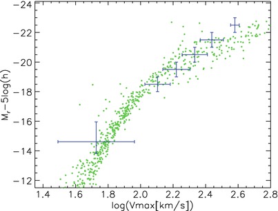
Fig. 10.35
The Tully–Fisher relation in the r-band.
Green points show the
absolute r-band magnitude of disk-dominated galaxies as a function
of maximum rotational velocity of their host halos, as obtained
from the same semi-analytic model as shown in Fig. 10.34. This is compared
to observational results indicated by the blue crosses. Semi-analytic models are
thus able to reproduce the zero point and approximate shape of the
Tully–Fisher relation over a range of about 8 magnitudes. Source:
Q. Guo et al. 2011, From
dwarf spheroidals to cD galaxies: simulating the galaxy population
in a ΛCDM cosmology, MNRAS 413, 101, p. 119, Fig. 13.
Reproduced by permission of Oxford University Press on behalf of
the Royal Astronomical Society
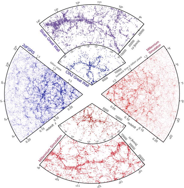
Fig. 10.36
Large-scale distribution of galaxies as
obtained from redshift surveys (in blue) and from semi-analytic models of
galaxies in the Millennium simulation (in red). On the left, one hemisphere of the 2dFGRS is
shown (cf. Fig. 7.1), whereas on the top the small wedge diagram shows the
CfA2 redshift survey (Fig. 7.2) with the Coma cluster at its
center, and the large wedge is part of the SDSS. In much the same
way as the observed distributions are obtained, the galaxy
distribution from the Millennium simulation has been transformed
into wedge diagrams shown in red. They are very similar to the
observed ones—they show great walls, fingers of god (since the
model galaxies are plotted in redshift space, as their peculiar
velocity is given by the simulation), as well as the cellular
structure of filaments and voids. Source: V. Springel et al.
2006, The large-scale structure of
the Universe, Nature 440, 1137, Fig. 1. Reprinted by
permission of Macmillan Publishers Ltd: Nature, ©2006
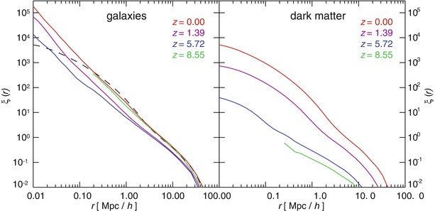
Fig. 10.37
The correlation function of galaxies
(left) and dark matter
(right) in the Millennium
simulation, for different redshifts. The dashed curve in the left panel shows the z = 0 dark matter correlation, for
easier comparison. The galaxies are selected above a given I-band
luminosity. There are striking differences between these two
correlations. As expected from structure growth, the dark matter
correlation function decreases with increasing redshift (remember,
on large scales where structure evolution follows linear
perturbation theory,  . In contrast to
that, the evolution of the galaxy correlation function is much
smaller, and it is not monotonic with redshift: the correlation at
the highest redshift is almost the same as the one at z = 0. Source: V. Springel et al.
2006, The large-scale structure of
the Universe, Nature 440, 1137, Fig. 5. Reprinted by
permission of Macmillan Publishers Ltd: Nature, ©2006
. In contrast to
that, the evolution of the galaxy correlation function is much
smaller, and it is not monotonic with redshift: the correlation at
the highest redshift is almost the same as the one at z = 0. Source: V. Springel et al.
2006, The large-scale structure of
the Universe, Nature 440, 1137, Fig. 5. Reprinted by
permission of Macmillan Publishers Ltd: Nature, ©2006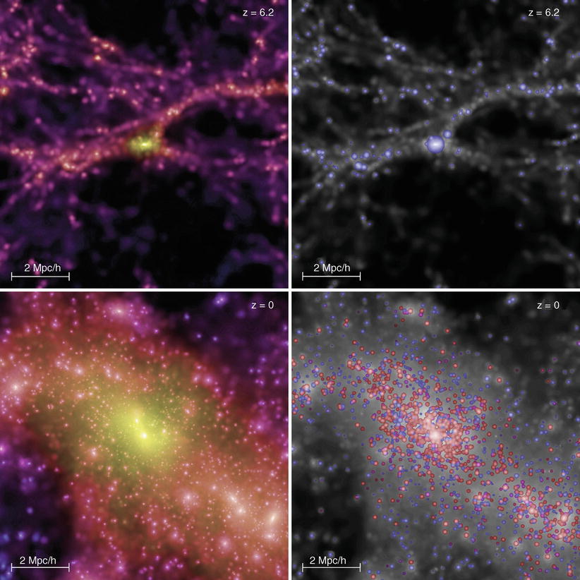
Fig. 10.38
In the top
panels, one of the most massive halos at z = 6. 2 from the Millennium simulation
(see Fig. 7.13) is shown, whereas in the
bottom panels, the
corresponding distribution in this spatial region at z = 0 is shown. Thus, this early
massive halo is now located in the center of a very massive galaxy
cluster. In the panels on the
left, the mass distribution is displayed. The corresponding
distribution of galaxies as determined from a semi-analytic model
is shown in the right-hand
panels. Galaxies at z = 6. 2 are all blue since their
stellar population must be young, whereas at z = 0, most galaxies contain an old
stellar population, here indicated by the red color. Each of the panels shows the
projected distribution of a cube with a comoving side length of
10 h −1 Mpc.
Source: V. Springel et al. 2005, Simulating the joint evolution of quasars,
galaxies and their large-scale distribution, Nature 435,
629, Fig. 3. Reprinted by permission of Macmillan Publishers Ltd:
Nature, ©2005
Spatial
distribution and correlation function. Since the spatial
location of the galaxies is known from such simulations, one can
compare their spatial distribution with that of the galaxies from
redshift surveys. This is illustrated in Fig. 10.36, which shows a
comparison of wedge diagrams from redshift surveys with those
obtained from the semi-analytic models applied to the dark matter
distribution of the Millennium simulation. At least at first sight,
the statistical properties of the ‘red’ and ‘blue’ wedge diagrams
are the same. The model predicts the occurrence of ‘Great Walls’,
as well as the system of voids and filaments in the overall galaxy
distribution. This comparison can be made more quantitative, for
example by comparing the two-point correlation function of model
galaxies with that obtained from observations. Also here, good
qualitative agreement is found, though the simulation slightly
overpredicts the amplitude of the correlation function. This,
however, may be due to the fact that the normalization of the power
spectrum was chosen to be σ
8 = 0. 9, slightly larger than the current best
estimates for our Universe (see Sect. 8.7).
The correlation function of galaxies has a rather
different behavior as a function of scale and redshift than that of
the dark matter. In Fig. 10.37, the correlation function of luminous
galaxies and that of the overall matter distribution is shown for
four different redshifts. Several issues are remarkable. First, the
dark matter correlation function ξ m(r) is not well approximated by a power
law, whereas the galaxy correlation function ξ g(r) shows a power-law behavior over many
decades of spatial scale, in agreement with observed galaxy
correlation functions. At z = 0 (red curve), ξ g(r) almost traces the correlation
function of matter on scales r ≳ 1h −1 Mpc, but they disagree
substantially on smaller scales. This implies that the bias of
galaxies is strongly scale-dependent, at least on small scales. In
fact, the question arises as to which processes in the evolution of
galaxies may produce such a perfect power law: why does the bias
factor behave just such that ξ g attains this simple
shape. The answer is found by analyzing galaxies with and without
active star formation separately; for each of these sub-populations
of galaxies, ξ g
is not a power law.
Therefore, the simple shape of the correlation function shown in
Fig. 10.37 is
probably a mere coincidence (‘cosmic conspiracy’).
Second, the matter correlation function strongly
decreases with increasing redshift, whereas ξ g evolves much slower with
z. This implies that the
bias of galaxies is redshift dependent; for a given galaxy
luminosity (or stellar mass), the bias increases with redshift. In
fact, we see that ξ
g at z = 8. 55
is almost identical with the one at zero redshift—the dependence of
ξ g on redshift
is not monotonic.
Early QSOs.
Another result from such models is presented in Fig. 10.38, also from the
Millennium simulation . Here, one of the most massive dark matter
halos in the simulation box at redshift z = 6. 2 is shown, together with the
mass distribution in this spatial region at redshift z = 0. In both cases, besides the
distribution of dark matter, the galaxy distribution is also
displayed, obtained from semi-analytic models. Massive halos which
have formed early in cosmic history are currently found
predominantly in the centers of very massive galaxy clusters.
Assuming that the luminous QSOs at z ∼ 6 are harbored in the most massive
halos of that epoch, we might suppose that these may today be
identified as the central galaxies in clusters.12 This may provide an explanation as
to why so many central, dominating cluster galaxies show AGN
activity, though with a smaller luminosity due to small accretion
rates.
From what we presented in this section, we can
summarize that semi-analytic modelling of galaxies is a very useful
method to make the link between the dark matter distribution on the
one hand, and the properties of the galaxy population on the other.
Since semi-analytic models are computational inexpensive, compared
to gas-dynamical simulations, one can experiment with them and
study in detail the dependence of galaxy properties on certain
assumptions and parameter choices. Furthermore, these models allow
us to include our best knowledge and understanding of the various
complex baryonic processes in a unified way which yields
quantitative results. We also have a fairly good understanding of
the mean properties of galaxies and their central black holes. Much
of this knowledge has been obtained only in recent years, and there
is no doubt that future observational results will lead to further
refinements, and perhaps qualitative modifications, of our
understanding.
Footnotes
1
Spectroscopy in the NIR is possible in principle,
but the high level of night-sky brightness and, in particular, the
large number of atmospheric transition lines renders spectroscopic
observations in the NIR much more time consuming than optical
spectroscopy.
2
To destroy all the H2 in the Universe
one needs less than 1 % of the photon flux that is required for the
reionization.
4
Note that in this case, the baryons are embedded
in a dark matter halo, so the consideration of the spin parameter,
which applies for the total energy and angular momentum, no longer
applies to the baryons only. Therefore, in this case (10.11) does not hold for
the baryons alone.
5
In this case of high collision velocity, the time
it takes a galaxy from one of the two clusters to cross the
gravitational potential of the other cluster is shorter than the
time it takes the matter of the second cluster to react to the
changing conditions caused by the merger; therefore, the
gravitational potential of the second cluster can be considered
almost stationary during the collision process. Thus, the galaxy
leaves the potential of the second cluster with almost the same
velocity it had on entering, i.e., it is not gravitationally bound
to the second cluster.
6
The fact that spectacular images of merging
galaxies show mainly gas-rich mergers (such as in Fig. 9.25 or 1.16) can be attributed to
selection effects. On the one hand, gas-rich mergers lead to
massive star formation, yielding a statistically increased
luminosity of the systems, whereas dry mergers basically preserve
the luminosity. On the other hand, gas-rich mergers can be
recognized as such for a longer period of time than dry ones, owing
to the clearly visible tidal tails traced by luminous newly formed
stars.
7
Calculating the behavior of a binary black, using
the equations of General Relativity, turns out to be very difficult
endeavor. Only since 2005 it has become possible to find numerical
solutions of this problem.
8
The equations of hydrodynamics describe the
behavior—or transport—of the mass, momentum and energy in a fluid.
Mass conservation is expressed by the continuity equation
(7.2). The evolution of the fluid
momentum is given, in the simplest case, by the Euler
equation (7.3); however, since gas is
dissipative, frictional terms need to be included (the resulting
equation for the fluid velocity is then called Navier–Stokes
equation). Finally, the transport of energy is described by an
energy equation, which contains sources and sinks of energy, as
they can be caused by absorption and emission of radiation and the
local generation of heat by frictional forces.
9
The situation is rather similar in meteorology,
where we believe to know all the essential physical processes that
affect the Earth atmosphere; nevertheless, we all know that weather
predictions can be terribly wrong, even on short time-scales. The
reason is that, although the relevant physical laws are known,
their consequences cannot be calculated with sufficient accuracy
due to the complexity of the underlying equations. Also in this
case, small-scale, highly non-linear processes (convection,
turbulence) have an impact on the large-scale properties of the
atmosphere.
10
In fact, one can obtain a statistical ensemble of
such merger trees also analytically from an extension of the
Press–Schechter theory (see Sect. 7.5.2),
but referring to N-body simulations also yields a prescription of
the spatial distribution of the resulting galaxy
distribution.
11
Of course, this simple picture ignores all the
difficulties in understanding the transport of gas from large
distances to the immediate vicinity of the black hole where it can
be accreted.