We will now begin to consider the Universe as a
whole. Individual objects such as galaxies and stars will no longer
be the subject of discussion, but instead we will turn our
attention to the space and time in which these objects are
embedded. These considerations will then lead to a world model, the
model of our cosmos. We need such a model also to interpret the
observations of distant objects, i.e., those with a redshift for
which the local Hubble law (1.2) ceases to be valid.
This chapter will deal with aspects of
homogeneous cosmology. As we will see, the Universe can, to first
approximation, be considered as being homogeneous. At first sight
this fact obviously seems to contradict observations because the
world around us is highly inhomogeneous and structured. Thus the
assumption of homogeneity is certainly not valid on small scales.
But observations are compatible with the assumption that the
Universe is homogeneous when averaged over large spatial scales.
Aspects of inhomogeneous cosmology, and thus the formation and
evolution of structures in the Universe, will be considered later
in Chap. 7.
4.1 Introduction and fundamental observations
Cosmology is a very special science indeed. To be
able to appreciate its peculiar role we should recall the typical
way of establishing knowledge in natural sciences. It normally
starts with the observation of some regular patterns, for instance
the observation that the height h a stone falls through is related
quadratically to the time t
it takes to fall,  . This relation is then also found
for other objects and observed at different places on Earth.
Therefore, this relation is formulated as the ‘law’ of free fall.
The constant of proportionality g∕2 in this law is always the same.
This law of physics is tested by its prediction of how an object
falls, and wherever this prediction is tested it is
confirmed—disregarding the resistance of air in this simple
example, of course.
. This relation is then also found
for other objects and observed at different places on Earth.
Therefore, this relation is formulated as the ‘law’ of free fall.
The constant of proportionality g∕2 in this law is always the same.
This law of physics is tested by its prediction of how an object
falls, and wherever this prediction is tested it is
confirmed—disregarding the resistance of air in this simple
example, of course.Relations become physical laws if the predictions
they make are confirmed again and again; the validity of such a law
is considered more secure the more diverse the tests have been. The
law of free fall was tested only on the surface of the Earth and it
is only valid there with this constant of proportionality.1 In contrast to this,
Newton’s law of gravity contains the law of free fall as a special
case, but it also describes the free fall on the surface of the
Moon, and the motion of planets around the Sun. If only a single
stone was available, we would not know whether the law of free fall
is a property of this particular stone or whether it is valid more
generally.
In some ways, cosmology corresponds to the latter
example: we have only one single Universe available for
observation. Relations that are found in our cosmos cannot be
verified in other universes. Thus it is not possible to consider
any property of our Universe as ‘typical’—we have no statistics on
which we could base a statement like this. Despite this special
situation, enormous progress has been made in understanding our
Universe, as we will describe here and in subsequent
chapters.
Cosmological observations are difficult in
general, simply because the majority of the Universe (and with it
most of the sources it contains) is very far away from us. Distant
sources are very dim. This explains why our knowledge of the
Universe runs in parallel with the development of large telescopes
and sensitive detectors. Much of today’s knowledge of the distant
Universe became available only with the new generation of optical
telescopes of the 8-m class, as well as new and powerful telescopes
in other wavelength regimes.
Fig. 4.1
The APM-survey: galaxy distribution in
a ∼ 100 × 50 degree2 field around the South Galactic
Pole. The intensities of the pixels are scaled with the number of
galaxies per pixel, i.e., the projected galaxy number density on
the sphere. The ‘holes’ are regions around bright stars, globular
clusters etc., that were not surveyed. Credit: S. Maddox,
W. Sutherland, G. Efstathiou & J. Loveday, with follow-up by
G. Dalton, and Astrophysics Dept., Oxford University
The most important aspect of cosmological
observations is the finite speed of light. We observe a source at
distance D in an
evolutionary state at which it was  younger than today. Thus we can
observe the current state of the Universe only very locally.
Another consequence of this effect, however, is of even greater
importance: due to the finite speed of light, it is possible to
look back into the past. At a distance of ten billion light years
we observe galaxies in an evolutionary state when the Universe had
only a third of its current age. Although we cannot observe the
past of our own Milky Way, we can study that of other galaxies. If
we are able to identify among them the ones that will form objects
similar to our Galaxy in the course of cosmic evolution, we will be
able to learn a great deal about the typical evolutionary history
of such spirals.
younger than today. Thus we can
observe the current state of the Universe only very locally.
Another consequence of this effect, however, is of even greater
importance: due to the finite speed of light, it is possible to
look back into the past. At a distance of ten billion light years
we observe galaxies in an evolutionary state when the Universe had
only a third of its current age. Although we cannot observe the
past of our own Milky Way, we can study that of other galaxies. If
we are able to identify among them the ones that will form objects
similar to our Galaxy in the course of cosmic evolution, we will be
able to learn a great deal about the typical evolutionary history
of such spirals.The finite speed of light in a Euclidean space,
in which we are located at the origin  today (t = t 0), implies that we can
only observe points in spacetime for which
today (t = t 0), implies that we can
only observe points in spacetime for which  ;
an arbitrary point
;
an arbitrary point  in spacetime is not observable.
The set of points in spacetime which satisfy the relation
in spacetime is not observable.
The set of points in spacetime which satisfy the relation
 is called our backward light
cone.
is called our backward light
cone.
today (t = t 0), implies that we can
only observe points in spacetime for which ;
an arbitrary point in spacetime is not observable.
The set of points in spacetime which satisfy the relation
is called our backward light
cone.The fact that our astronomical observations are
restricted to sources which are located on our backward light cone
implies that our possibilities to observe the Universe are
fundamentally limited. If somewhere in spacetime there would be a
highly unusual event, we will not be able to observe it unless it
happens to lie on our backward light cone. Only if the Universe has
an essentially ‘simple’ structure will we be able to understand it,
by combining astronomical observations with theoretical modeling.
Luckily, our Universe seems to be basically simple in this
sense.
4.1.1 Fundamental cosmological observations
We will begin with a short list of key
observations that have proven to be of particular importance for
cosmology. Using these observational facts we will then be able to
draw a number of immediate conclusions; other observations will be
explained later in the context of a cosmological model.
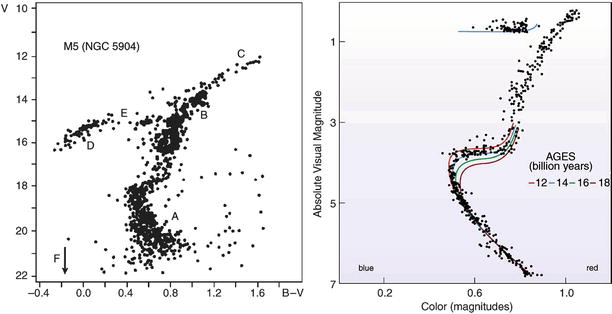
Fig. 4.2
Left
panel: Color-magnitude diagram of the globular cluster M 5.
The different sections in this diagram are labeled. A: main
sequence; B: red giant branch; C: point of helium flash; D:
horizontal branch; E: Schwarzschild-gap in the horizontal branch;
F: white dwarfs, below the arrow. At the point where the main
sequence turns over to the red giant branch (called the ‘turn-off
point’), stars have a mass corresponding to a main-sequence
lifetime which is equal to the age of the globular cluster (see
Appendix B.3). Therefore, the age of the cluster can be determined
from the position of the turn-off point by comparing it with models
of stellar evolution. Right
panel: Isochrones, i.e., curves connecting the stellar
evolutionary position in the color-magnitude diagram of stars of
equal age, are plotted for different ages and compared to the stars
of the globular cluster 47 Tucanae. Such analyses reveal that the
oldest globular clusters in our Milky Way are about 12 billion
years old, where different authors obtain slightly differing
results—details of stellar evolution may play a role here. The age
thus obtained also depends on the distance of the cluster. A
revision of these distances by the Hipparcos satellite led to a
decrease of the estimated ages by about two billion years. Credit:
M5: ©Leos Ondra; 47 Tuc: J.E. Hesser, W.E. Harris, D.A. Vandenberg,
J.W.B. Allwright, P. Scott & P.B. Stetson 1987, A CCD color-magnitude study of 47
Tucanae, PASP 99, 739
1.
The sky is dark at night (Olbers’ paradox).
2.
Averaged over large angular scales, faint
galaxies (e.g., those with R > 20) are uniformly distributed on
the sky (see Fig. 4.1).
3.
With the exception of a very few very nearby
galaxies (e.g., Andromeda = M31), a redshift is observed in the
spectra of galaxies—most galaxies are moving away from us, and
their escape velocity increases linearly with distance (Hubble law;
see Fig. 1.13).
4.
In nearly all cosmic objects (e.g., gas nebulae,
main sequence stars), the mass fraction of helium is 25–30 %.
6.
A microwave radiation (cosmic microwave
background radiation, CMB) is observed, reaching us from all
directions. This radiation is isotropic except for very small, but
immensely important, fluctuations with relative
amplitude ∼ 10−5 (see Fig. 1.21).
7.
The spectrum of the CMB corresponds, within the
very small error bars that were obtained by the measurements with
COBE, to that of a perfect blackbody, i.e., a Planck radiation of a
temperature of T
0 = 2. 728 ± 0. 004 K—see Fig. 4.3.
8.
The number counts of radio sources at high
Galactic latitude does not
follow the simple law  (see Fig. 4.4).
(see Fig. 4.4).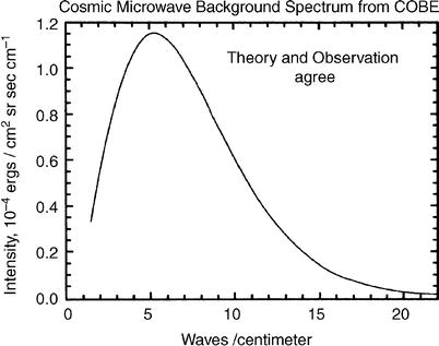
Fig. 4.3
CMB spectrum, plotted as intensity vs.
frequency, measured in waves per centimeter. The solid line shows the expected spectrum
of a blackbody of temperature T = 2. 728 K. The error bars of the
data, observed by the FIRAS instrument on-board COBE, are so small
that the data points with error bars cannot be distinguished from
the theoretical curve. Credit: COBE, NASA. We acknowledge the use
of the Legacy Archive for Microwave Data Analysis (LAMBDA). Support
for LAMBDA is provided by the NASA Office for Space Science
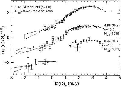
Fig. 4.4
Number counts of radio sources as a
function of their flux, normalized by the Euclidean expectation
 , corresponding to the
integrated counts
, corresponding to the
integrated counts  . Counts are displayed
for three different frequencies; they clearly deviate from the
Euclidean expectation. Source: R.A. Windhorst et al. 1993,
Microjansky source counts and
spectral indices at 8.44 GHz, ApJ 405, 498, p. 508, Fig. 3.
©AAS. Reproduced with permission
. Counts are displayed
for three different frequencies; they clearly deviate from the
Euclidean expectation. Source: R.A. Windhorst et al. 1993,
Microjansky source counts and
spectral indices at 8.44 GHz, ApJ 405, 498, p. 508, Fig. 3.
©AAS. Reproduced with permission
, corresponding to the
integrated counts . Counts are displayed
for three different frequencies; they clearly deviate from the
Euclidean expectation. Source: R.A. Windhorst et al. 1993,
Microjansky source counts and
spectral indices at 8.44 GHz, ApJ 405, 498, p. 508, Fig. 3.
©AAS. Reproduced with permission4.1.2 Simple conclusions
We will next draw a number of simple conclusions
from the observational facts listed above. These will then serve as
a motivation and guideline for developing the cosmological model.
We will start with the assumption of an infinite, on-average
homogeneous, Euclidean, static universe, and show that this
assumption is in direct contradiction to observations (1) and
(8).
Olbers’ paradox
(1): We can show that the night sky would be bright in such
a universe—uncomfortably bright, in fact. Let n ∗ be the mean number
density of stars, constant in space and time according to the
assumptions, and let R
∗ be their mean radius. A spherical shell of radius
r and thickness
dr around us contains
 stars. Each of these stars subtends a solid angle of π R ∗
2∕r 2
on our sky, so the stars in the shell cover a total solid angle of
stars. Each of these stars subtends a solid angle of π R ∗
2∕r 2
on our sky, so the stars in the shell cover a total solid angle of
 We see that this solid angle is independent of the radius
r of the spherical shell
because the solid angle covered by a single star
We see that this solid angle is independent of the radius
r of the spherical shell
because the solid angle covered by a single star  just compensates the volume of the
shell ∝ r 2. To
compute the total solid angle of all stars in a static Euclidean
universe, (4.1) has to be integrated over all distances
r, but the integral
just compensates the volume of the
shell ∝ r 2. To
compute the total solid angle of all stars in a static Euclidean
universe, (4.1) has to be integrated over all distances
r, but the integral
 diverges. Formally, this means that the stars cover an infinite
solid angle, which of course makes no sense physically. The reason
for this divergence is that we disregarded the effect of
overlapping stellar disks on the sphere. However, these
considerations demonstrate that the sky would be completely filled
with stellar disks, i.e., from any direction, along any
line-of-sight, light from a stellar surface would reach us. Since
the specific intensity I
ν is independent
of distance—the surface brightness of the Sun as observed from
Earth is the same as seen by an observer who is much closer to the
Solar surface—the sky would have a temperature
of ∼ 104 K; fortunately, this is not the case!
diverges. Formally, this means that the stars cover an infinite
solid angle, which of course makes no sense physically. The reason
for this divergence is that we disregarded the effect of
overlapping stellar disks on the sphere. However, these
considerations demonstrate that the sky would be completely filled
with stellar disks, i.e., from any direction, along any
line-of-sight, light from a stellar surface would reach us. Since
the specific intensity I
ν is independent
of distance—the surface brightness of the Sun as observed from
Earth is the same as seen by an observer who is much closer to the
Solar surface—the sky would have a temperature
of ∼ 104 K; fortunately, this is not the case!
stars. Each of these stars subtends a solid angle of π R ∗
2∕r 2
on our sky, so the stars in the shell cover a total solid angle of
(4.1)
just compensates the volume of the
shell ∝ r 2. To
compute the total solid angle of all stars in a static Euclidean
universe, (4.1) has to be integrated over all distances
r, but the integral
Source counts
(8): Consider now a population of sources with a luminosity
function that is constant in space and time, i.e., let n( > L) be the spatial number density of
sources with luminosity larger than L. A spherical shell of radius
r and thickness
dr around us contains
4π r
2 dr n( > L)
sources with luminosity larger than L. Because the observed flux
S is related to the
luminosity via L = 4π r 2 S, the number of sources with
flux > S in this
spherical shell is given as  ,
and the total number of sources with flux > S results from integration over the
radii of the spherical shells,
,
and the total number of sources with flux > S results from integration over the
radii of the spherical shells,
 Changing the integration variable to L = 4π r 2 S, or
  , with
  , yields
 From this result we deduce that the source counts in such a
universe is
From this result we deduce that the source counts in such a
universe is  , independent of the
luminosity function. This is in contradiction to the
observations.
, independent of the
luminosity function. This is in contradiction to the
observations.
,
and the total number of sources with flux > S results from integration over the
radii of the spherical shells,
, with , yields
(4.2)
, independent of the
luminosity function. This is in contradiction to the
observations.From these two contradictions—Olbers’ paradox and
the non-Euclidean source counts—we conclude that at least one of
the assumptions must be wrong. Our Universe cannot be all four of
Euclidean, homogeneous, infinite, and static. The Hubble flow,
i.e., the redshift of galaxies, indicates that the assumption of a
static Universe is wrong.
The age of
globular clusters (5) requires that the Universe is at least
12 Gyr old because it cannot be younger than the oldest objects it
contains. Interestingly, the age estimates for globular clusters
yield values which are very close to the Hubble time  . This
similarity suggests that the Hubble expansion may be directly
linked to the evolution of the Universe.
. This
similarity suggests that the Hubble expansion may be directly
linked to the evolution of the Universe.
. This
similarity suggests that the Hubble expansion may be directly
linked to the evolution of the Universe.The apparently isotropic distribution of galaxies (2), when
averaged over large scales, and the CMB isotropy (6) suggest that the
Universe around us is isotropic on large angular scales. Therefore
we will first consider a world model that describes the Universe
around us as isotropic. If we assume, in addition, that our place
in the cosmos is not privileged over any other place, then the
assumption of isotropy around us implies that the Universe appears
isotropic as seen from any other place. The homogeneity of the
Universe follows immediately from the isotropy around every
location, as explained in Fig. 4.5. The combined assumption of homogeneity and
isotropy of the Universe is also known as the cosmological principle. We will see
that a world model based on the cosmological principle in fact
provides an excellent description of numerous observational
facts.
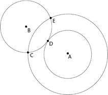
Fig. 4.5
Homogeneity follows from the isotropy
around two points. If the Universe is isotropic around observer B,
the densities at C, D, and E are equal. Drawing spheres of
different radii around observer A, it is seen that the region
within the spherical shell around A has to be homogeneous. By
varying the radius of the shell, we can conclude the whole Universe
must be homogeneous. Credit: J.A. Peacock 1999, Cosmological Physics, Cambridge
University Press
However, homogeneity is in principle unobservable
because observations of distant objects show those at an earlier
epoch. If the Universe evolves in time, as the aforementioned
observations suggest, evolutionary effects cannot directly be
separated from spatial variations.
The assumption of homogeneity of course breaks
down on small scales. We observe structures in the Universe, like
galaxies and clusters of galaxies, and even accumulations of
clusters of galaxies, so-called superclusters. Structures have been
found in redshift surveys that extend over ∼ 100 h −1 Mpc. However, we have
no indication of the existence of structures in the Universe with
scales  . This length-scale
can be compared to a characteristic length of the Universe, which
is obtained from the Hubble constant. If H 0 −1 specifies
the characteristic age of our Universe, then light will travel a
distance c∕H 0 in this time. With this,
we have obtained in problem 1.1 the Hubble radius as a characteristic
length-scale of the Universe (or more precisely, of the observable
Universe),
. This length-scale
can be compared to a characteristic length of the Universe, which
is obtained from the Hubble constant. If H 0 −1 specifies
the characteristic age of our Universe, then light will travel a
distance c∕H 0 in this time. With this,
we have obtained in problem 1.1 the Hubble radius as a characteristic
length-scale of the Universe (or more precisely, of the observable
Universe),
 The Hubble volume ∼ R
H 3 can contain a very large number of
structures of size ∼ 100 h
−1 Mpc, so that it still makes sense to assume an
on-average homogeneous cosmological model. Superposed on this
homogeneous universe we then have density fluctuations that are
identified with the observed large-scale structures; these will be
discussed in detail in Chap. 7. To a first approximation we can
neglect these density perturbations in a description of the
Universe as a whole. We will therefore consider world models that
are based on the cosmological principle, i.e., in which the
universe looks the same for all observers (or, in other words, if
observed from any point).
The Hubble volume ∼ R
H 3 can contain a very large number of
structures of size ∼ 100 h
−1 Mpc, so that it still makes sense to assume an
on-average homogeneous cosmological model. Superposed on this
homogeneous universe we then have density fluctuations that are
identified with the observed large-scale structures; these will be
discussed in detail in Chap. 7. To a first approximation we can
neglect these density perturbations in a description of the
Universe as a whole. We will therefore consider world models that
are based on the cosmological principle, i.e., in which the
universe looks the same for all observers (or, in other words, if
observed from any point).
. This length-scale
can be compared to a characteristic length of the Universe, which
is obtained from the Hubble constant. If H 0 −1 specifies
the characteristic age of our Universe, then light will travel a
distance c∕H 0 in this time. With this,
we have obtained in problem 1.1 the Hubble radius as a characteristic
length-scale of the Universe (or more precisely, of the observable
Universe),
(4.3)
Homogeneous and isotropic world models are the
simplest cosmological solutions of the equations of General
Relativity (GR). We will examine how far such simple models are
compatible with observations. As we shall see, the application of
the cosmological principle results in the observational facts which
were mentioned in Sect. 4.1.1.
4.2 An expanding universe
Gravitation is the fundamental force in the
Universe. Only gravitational forces and electromagnetic forces can
act over large distance. Since cosmic matter is electrically
neutral on average, electromagnetic forces do not play any
significant role on large scales, so that gravity has to be
considered as the driving force in cosmology. The laws of gravity
are described by the theory of General Relativity, formulated by A.
Einstein in 1915. It contains Newton’s theory of gravitation as a
special case for weak gravitational fields and small spatial
scales. Newton’s theory of gravitation has been proven to be
eminently successful, e.g., in describing the motion of planets.
Thus it is tempting to try to design a cosmological model based on
Newtonian gravity. We will proceed to do that as a first step
because not only is this Newtonian cosmology very useful from a
didactic point of view, but one can also argue why the Newtonian
cosmos correctly describes the major aspects of a relativistic
cosmology.
4.2.1 Newtonian cosmology
The description of a gravitational system
necessitates the application of GR if the length-scales in the
system are comparable to the radius of curvature of spacetime; this
is certainly the case in our Universe. Even if we cannot explain at
this point what exactly the ‘curvature radius of the Universe’ is,
it should be plausible that it is of the same order of magnitude as
the Hubble radius R
H. We will discuss this more thoroughly further below.
Despite this fact, one can expect that a Newtonian description is
essentially correct: in a homogeneous universe, any small spatial
region is characteristic for the whole universe. If the evolution
of a small region in space is known, we also know the history of
the whole universe, due to homogeneity. However, on small scales,
the Newtonian approach is justified. We will therefore, based on
the cosmological principle, first consider spatially homogeneous
and isotropic world models in the framework of Newtonian
gravity.
4.2.2 Kinematics of the Universe
Comoving
coordinates. We consider a homogeneous sphere which may be
radially expanding (or contracting); however, we require that the
density ρ(t) remains spatially homogeneous. The
density may vary in time due to expansion or contraction. We choose
a point t = t 0 in time and introduce a
coordinate system  at this instant with the origin
coinciding with the center of the sphere. A particle in the sphere
which is located at position
at this instant with the origin
coinciding with the center of the sphere. A particle in the sphere
which is located at position  at time t 0 will be located at some
other time t at the
position
at time t 0 will be located at some
other time t at the
position  which results from the expansion
of the sphere. Since the expansion is radial or, in other words,
the velocity vector of a particle at position
which results from the expansion
of the sphere. Since the expansion is radial or, in other words,
the velocity vector of a particle at position  is parallel to
  , the direction of
  is constant. Because
 , this means
that
, this means
that
 Since
Since  and
and  both have the dimension of a
length, the function a(t) is dimensionless; it can depend only
on time. Although requiring radial expansion alone could make
a depend on
both have the dimension of a
length, the function a(t) is dimensionless; it can depend only
on time. Although requiring radial expansion alone could make
a depend on  as well, the
requirement that the density remains homogeneous implies that
a must be spatially
constant. The function a(t) is called the cosmic scale factor ; due to
as well, the
requirement that the density remains homogeneous implies that
a must be spatially
constant. The function a(t) is called the cosmic scale factor ; due to
 , it obeys
 The value of t 0
is arbitrary; we choose t
0 = today. Particles (or observers) which move according
to (4.4)
are called comoving particles
(observers), and
The value of t 0
is arbitrary; we choose t
0 = today. Particles (or observers) which move according
to (4.4)
are called comoving particles
(observers), and  is the comoving coordinate. The
world line
is the comoving coordinate. The
world line  of a comoving observer is
unambiguously determined by
of a comoving observer is
unambiguously determined by  ,
, ![$$({\boldsymbol r},t) = [a(t){\boldsymbol x},t]$$](A129044_2_En_4_Chapter_IEq32.gif) .
.
at this instant with the origin
coinciding with the center of the sphere. A particle in the sphere
which is located at position at time t 0 will be located at some
other time t at the
position which results from the expansion
of the sphere. Since the expansion is radial or, in other words,
the velocity vector of a particle at position is parallel to , the direction of is constant. Because
, this means
that
(4.4)
and both have the dimension of a
length, the function a(t) is dimensionless; it can depend only
on time. Although requiring radial expansion alone could make
a depend on as well, the
requirement that the density remains homogeneous implies that
a must be spatially
constant. The function a(t) is called the cosmic scale factor ; due to
, it obeys
(4.5)
is the comoving coordinate. The
world line of a comoving observer is
unambiguously determined by , .Expansion
rate. The velocity of such a comoving particle is obtained
from the time derivative of its position,
 where in the last step we defined the expansion rate
 The choice of this notation is not accidental, since H is closely related to the Hubble
constant. To see this, we consider the relative velocity vector of
two comoving particles at positions
The choice of this notation is not accidental, since H is closely related to the Hubble
constant. To see this, we consider the relative velocity vector of
two comoving particles at positions  and
and  , which
follows directly from (4.6):
, which
follows directly from (4.6):
 Hence, the relative velocity is proportional to the separation
vector, so that the relative velocity is purely radial.
Furthermore, the constant of proportionality H(t) depends only on time but not on the
position of the two particles. Obviously, (4.8) is very similar to
the Hubble law
Hence, the relative velocity is proportional to the separation
vector, so that the relative velocity is purely radial.
Furthermore, the constant of proportionality H(t) depends only on time but not on the
position of the two particles. Obviously, (4.8) is very similar to
the Hubble law
 in which v is the radial
velocity of a source at distance D from us. Therefore, setting
t = t 0 and H 0 ≡ H(t 0), (4.8) is simply the Hubble
law, in other words, (4.8) is a generalization of (4.9) for arbitrary time.
It expresses the fact that any observer expanding with the sphere
will observe an isotropic velocity field that follows the Hubble
law. Since we are observing an expansion today—sources are moving
away from us—we have H
0 > 0, and
in which v is the radial
velocity of a source at distance D from us. Therefore, setting
t = t 0 and H 0 ≡ H(t 0), (4.8) is simply the Hubble
law, in other words, (4.8) is a generalization of (4.9) for arbitrary time.
It expresses the fact that any observer expanding with the sphere
will observe an isotropic velocity field that follows the Hubble
law. Since we are observing an expansion today—sources are moving
away from us—we have H
0 > 0, and  .
.
(4.6)
(4.7)
and , which
follows directly from (4.6):
(4.8)
(4.9)
.The kinematics of comoving observers in an
expanding universe is analogous to that of raisins in a yeast
dough. Once in the oven, the dough expands, and accordingly the
positions of the raisins change. All raisins move away from all
other ones, and the mutual radial velocity is proportional to the
separation between any pair of raisins—i.e., their motion follows
the Hubble law (4.8), with an expansion rate H(t) which depends on the quality of the
yeast and the temperature of the oven. The spatial position of each
raisin at the time the oven is started uniquely identifies a
raisin, and can be taken as its comoving coordinate  , measured relative to the center of
the dough. The spatial position
, measured relative to the center of
the dough. The spatial position  at some later time t is then given by (4.4), where a(t) denotes the linear size of the dough
at time t relative to the
size when the oven was started.
at some later time t is then given by (4.4), where a(t) denotes the linear size of the dough
at time t relative to the
size when the oven was started.
, measured relative to the center of
the dough. The spatial position at some later time t is then given by (4.4), where a(t) denotes the linear size of the dough
at time t relative to the
size when the oven was started.4.2.3 Dynamics of the expansion
The above discussion describes the kinematics of
the expansion. However, to obtain the behavior of the function
a(t) in time, and thus also the motion of
comoving observers and the time evolution of the density of the
sphere, it is necessary to consider the dynamics. The evolution of
the expansion rate is determined by self-gravity of the sphere,
from which it is expected that it will cause a deceleration of the
expansion.
Equation of
motion. We therefore consider a spherical surface of radius
x at time t 0 and, accordingly, a
radius r(t) = a(t) x at arbitrary time t. The mass M(x) enclosed in this comoving surface is
constant in time, and is given by
 where ρ 0 must
be identified with the mass density of the universe today
(t = t 0). The density is a
function of time and, due to mass conservation, it is inversely
proportional to the volume of the sphere,
where ρ 0 must
be identified with the mass density of the universe today
(t = t 0). The density is a
function of time and, due to mass conservation, it is inversely
proportional to the volume of the sphere,
 The gravitational acceleration of a particle on the spherical
surface is GM(x)∕r 2, directed towards the
center. This then yields the equation of motion of the particle,
The gravitational acceleration of a particle on the spherical
surface is GM(x)∕r 2, directed towards the
center. This then yields the equation of motion of the particle,
 or, after substituting r(t) = x a(t), an equation for a ,
 It is important to note that this equation of motion does not
dependent on x. The
dynamics of the expansion, described by a(t), is determined solely by the matter
density.
It is important to note that this equation of motion does not
dependent on x. The
dynamics of the expansion, described by a(t), is determined solely by the matter
density.
(4.10)
(4.11)
(4.12)
(4.13)
‘Conservation of
energy’. Another way to describe the dynamics of the
expanding shell is based on the law of energy conservation: the sum
of kinetic and potential energy is constant in time. This
conservation of energy is derived directly from (4.13). To do
this, (4.13) is multiplied by  ,
and the resulting equation can be integrated with respect to time
since
,
and the resulting equation can be integrated with respect to time
since  ,
and
,
and  :
:
 here, Kc 2 is a
constant of integration that will be interpreted later. After
multiplication with x
2∕2, (4.14) can be written as
here, Kc 2 is a
constant of integration that will be interpreted later. After
multiplication with x
2∕2, (4.14) can be written as
 which is interpreted such that the kinetic + potential energy (per
unit mass) of a particle is a constant on the spherical surface.
Thus (4.14) in fact describes the conservation of
energy. The latter equation also immediately suggests an
interpretation of the integration constant: K is proportional to the total energy
of a comoving particle, and thus the history of the expansion
depends on K. The sign of
K characterizes the
qualitative behavior of the cosmic expansion history.
which is interpreted such that the kinetic + potential energy (per
unit mass) of a particle is a constant on the spherical surface.
Thus (4.14) in fact describes the conservation of
energy. The latter equation also immediately suggests an
interpretation of the integration constant: K is proportional to the total energy
of a comoving particle, and thus the history of the expansion
depends on K. The sign of
K characterizes the
qualitative behavior of the cosmic expansion history.
,
and the resulting equation can be integrated with respect to time
since ,
and :
(4.14)
-
If K < 0, the right-hand side of (4.14) is always positive. Since da∕dt > 0 today, da∕dt remains positive for all times or, in other words, the universe will expand forever.
-
If K = 0, the right-hand side of (4.14) is always positive, i.e., da∕dt > 0 for all times, and the universe will also expand forever, but in a way that da∕dt → 0 for t → ∞—the asymptotic expansion velocity for t → ∞ is zero.
-
If K > 0, the right-hand side of (4.14) vanishes if
 .
For this value of a,
.
For this value of a,
 , and the expansion will
come to a halt. After that, the expansion will turn into a
contraction, and such a universe will re-collapse.
, and the expansion will
come to a halt. After that, the expansion will turn into a
contraction, and such a universe will re-collapse.
In the special case of K = 0, which separates eternally
expanding world models from those that will re-collapse in the
future, the universe has a current density called critical density which can be inferred
from (4.14) by setting t = t 0 and  :
:
 Obviously, ρ cr
is a characteristic density of the current universe. As in many
situations in physics, it is useful to express physical quantities
in terms of dimensionless parameters, for instance the current
cosmological density. We therefore define the density parameter
Obviously, ρ cr
is a characteristic density of the current universe. As in many
situations in physics, it is useful to express physical quantities
in terms of dimensionless parameters, for instance the current
cosmological density. We therefore define the density parameter
 where K > 0 corresponds
to Ω 0 > 1,
and K < 0 corresponds to
Ω 0 < 1.
Thus, Ω 0 is one
of the central cosmological parameters. Its accurate determination
was possible only quite recently, and we shall discuss this in
detail later. However, we should mention here that matter which is
visible as stars contributes only a small fraction to the density
of our Universe,
where K > 0 corresponds
to Ω 0 > 1,
and K < 0 corresponds to
Ω 0 < 1.
Thus, Ω 0 is one
of the central cosmological parameters. Its accurate determination
was possible only quite recently, and we shall discuss this in
detail later. However, we should mention here that matter which is
visible as stars contributes only a small fraction to the density
of our Universe,  . But, as we
already discussed in the context of rotation curves of spiral
galaxies and the mass determination of elliptical galaxies from the
gravitational lensing effect, we find clear indications of the
presence of dark matter which can in principle dominate the value
of Ω 0. We will
see that this is indeed the case.
. But, as we
already discussed in the context of rotation curves of spiral
galaxies and the mass determination of elliptical galaxies from the
gravitational lensing effect, we find clear indications of the
presence of dark matter which can in principle dominate the value
of Ω 0. We will
see that this is indeed the case.
:
(4.15)
(4.16)
. But, as we
already discussed in the context of rotation curves of spiral
galaxies and the mass determination of elliptical galaxies from the
gravitational lensing effect, we find clear indications of the
presence of dark matter which can in principle dominate the value
of Ω 0. We will
see that this is indeed the case.4.2.4 Modifications due to General Relativity
The Newtonian approach contains nearly all
essential aspects of homogeneous and isotropic world models,
otherwise we would not have discussed it in detail. Most of the
above equations are also valid in relativistic cosmology, although
the interpretation needs to be altered. In particular, the image of
an expanding sphere needs to be revised—this picture implies that a
‘center’ of the universe exists. Such a picture implicitly
contradicts the cosmological principle in which no point is singled
out over others—our Universe neither has a center, nor is it
expanding away from a privileged point. However, the image of a
sphere does not show up in any of the relevant equations:
(4.11) for
the evolution of the cosmological density and (4.13)
and (4.14) for the evolution of the scale factor
a(t) contain no quantities that refer to
a sphere.
General Relativity modifies the Newtonian model
in several respects:
-
We know from the theory of Special Relativity that mass and energy are equivalent, according to Einstein’s famous relation E = m c 2. This implies that it is not only the matter density that contributes to the equations of motion. For example, a radiation field like the CMB has an energy density and, due to the equivalence above, this has to enter the expansion equations. We will see below that such a radiation field can be characterized as matter with pressure. The pressure will then explicitly appear in the equation of motion for a(t).
-
The field equation of GR as originally formulated by Einstein did not permit a solution which corresponds to a homogeneous, isotropic, and static cosmos. But since Einstein, like most of his contemporaries, believed the Universe to be static, he modified his field equations by introducing an additional term, the cosmological constant.
-
The interpretation of the expansion is changed completely: it is not the particles or the observers that are expanding away from each other, nor is the Universe an expanding sphere. Instead, it is space itself that expands. In particular, the redshift is no Doppler redshift, but is itself a property of expanding spacetimes. However, we may still visualize redshift locally as being due to the Doppler effect without making a substantial conceptual error.2
In the following, we will explain the first two
aspects in more detail.
First law of
thermodynamics. When air is compressed, for instance when
pumping up a tire, it heats up. The temperature increases and
accordingly so does the thermal energy of the air. In the language
of thermodynamics, this fact is described by the first law: the
change in internal energy dU through an (adiabatic) change in
volume dV equals the work
 , where P is the pressure in the gas. From the
equations of GR as applied to a homogeneous isotropic cosmos, a
relation is derived which reads
, where P is the pressure in the gas. From the
equations of GR as applied to a homogeneous isotropic cosmos, a
relation is derived which reads
 in full analogy to this law. Here, ρ c 2 is the energy density,
i.e., for ‘normal’ matter, ρ is the mass density, and P is the pressure of the matter. If we
now consider a constant comoving volume element V x , then its physical volume
V = a 3(t)V x will change due to expansion.
Thus,
in full analogy to this law. Here, ρ c 2 is the energy density,
i.e., for ‘normal’ matter, ρ is the mass density, and P is the pressure of the matter. If we
now consider a constant comoving volume element V x , then its physical volume
V = a 3(t)V x will change due to expansion.
Thus,  is the volume, and c 2 ρ a 3 the energy contained in
the volume, each divided by V x . Taken
together, (4.17) corresponds to the first law of
thermodynamics in an expanding universe.
is the volume, and c 2 ρ a 3 the energy contained in
the volume, each divided by V x . Taken
together, (4.17) corresponds to the first law of
thermodynamics in an expanding universe.
, where P is the pressure in the gas. From the
equations of GR as applied to a homogeneous isotropic cosmos, a
relation is derived which reads
(4.17)
is the volume, and c 2 ρ a 3 the energy contained in
the volume, each divided by V x . Taken
together, (4.17) corresponds to the first law of
thermodynamics in an expanding universe.The
Friedmann–Lemaître expansion equations. Next, we will
present equations for the scale factor a(t) which follow from GR for a
homogeneous isotropic universe. Afterwards, we will derive these
equations from the relations stated above—as we shall see, the
modifications by GR are in fact only minor, as expected from the
argument that a small section of a homogeneous universe
characterizes the cosmos as a whole. The field equations of GR
yield the equations of motion
 and
and
 where Λ is the
aforementioned cosmological constant introduced by
Einstein.3 Compared
to (4.13)
and (4.14), these two equations have been changed in
two places. First, the cosmological constant occurs in both
equations, and second, the equation of motion (4.19) now contains a
pressure term. The pair of (4.18) and (4.19) are called the
Friedmann equations.
where Λ is the
aforementioned cosmological constant introduced by
Einstein.3 Compared
to (4.13)
and (4.14), these two equations have been changed in
two places. First, the cosmological constant occurs in both
equations, and second, the equation of motion (4.19) now contains a
pressure term. The pair of (4.18) and (4.19) are called the
Friedmann equations.
(4.18)
(4.19)
The cosmological
constant. When Einstein introduced the Λ-term into his equations, he did this
solely for the purpose of obtaining a static solution for the
resulting expansion equations. We can easily see
that (4.18) and (4.19), without the
Λ-term, have no solution
for  . However, if the Λ-term is included, such a solution can
be found (which is irrelevant, however, as we now know that the
Universe is expanding). Einstein had no real physical
interpretation for this constant, and after the expansion of the
Universe was discovered he discarded it again. But with the genie
out of the bottle, the cosmological constant remained in the minds
of cosmologists, and their attitude towards Λ has changed frequently in the past 90
years. Around the turn of the millennium, observations were made
which strongly suggest a non-vanishing cosmological constant, and
the evidence has been further strengthened since, as will be
detailed in Chap. 8. Today we know that our Universe
has a non-zero cosmological constant, or at least something very
similar to it.
. However, if the Λ-term is included, such a solution can
be found (which is irrelevant, however, as we now know that the
Universe is expanding). Einstein had no real physical
interpretation for this constant, and after the expansion of the
Universe was discovered he discarded it again. But with the genie
out of the bottle, the cosmological constant remained in the minds
of cosmologists, and their attitude towards Λ has changed frequently in the past 90
years. Around the turn of the millennium, observations were made
which strongly suggest a non-vanishing cosmological constant, and
the evidence has been further strengthened since, as will be
detailed in Chap. 8. Today we know that our Universe
has a non-zero cosmological constant, or at least something very
similar to it.But the physical interpretation of the
cosmological constant has also been modified. In quantum mechanics
even completely empty space, the so-called vacuum, may have a
finite energy density, the vacuum energy density. For physical
measurements not involving gravity, the value of this vacuum energy
density is of no relevance since those measurements are only
sensitive to energy differences. For example, the energy of
a photon that is emitted in an atomic transition equals the energy
difference between the two corresponding states in the atom. Thus
the absolute energy of a state is measurable only up to a constant.
Only in gravity does the absolute energy become important, because
E = m c 2 implies that it
corresponds to a mass.
It is now found that the cosmological constant is
equivalent to a finite vacuum energy density—the equations of GR,
and thus also the expansion equations, are not affected by this new
interpretation. We will explain this fact in the following.
4.2.5 The components of matter in the Universe
Starting from the equation of energy
conservation (4.14), we will now derive the relativistically
correct expansion equations (4.18)
and (4.19). The only change with respect to the
Newtonian approach in Sect. 4.2.3 will be that we introduce other forms of
matter. The essential components of our Universe can be described
as pressure-free matter, radiation, and vacuum energy.
Pressure-free
matter. The pressure in a gas is determined by the thermal
motion of its constituents. At room temperature, molecules in the
air move at a speed comparable to the speed of sound,  . For such a
gas,
. For such a
gas,  ,
so that its pressure is of course gravitationally completely
insignificant. In cosmology, a substance with P ≪ ρ
c 2 is denoted as (pressure-free) matter, also
called cosmological dust.4We approximate P m = 0, where the index ‘m’
stands for matter. The constituents of the (pressure-free) matter
move with velocities much smaller than c.
,
so that its pressure is of course gravitationally completely
insignificant. In cosmology, a substance with P ≪ ρ
c 2 is denoted as (pressure-free) matter, also
called cosmological dust.4We approximate P m = 0, where the index ‘m’
stands for matter. The constituents of the (pressure-free) matter
move with velocities much smaller than c.
. For such a
gas, ,
so that its pressure is of course gravitationally completely
insignificant. In cosmology, a substance with P ≪ ρ
c 2 is denoted as (pressure-free) matter, also
called cosmological dust.4We approximate P m = 0, where the index ‘m’
stands for matter. The constituents of the (pressure-free) matter
move with velocities much smaller than c.Radiation.
If this condition is no longer satisfied, thus if the thermal
velocities are no longer negligible compared to the speed of light,
then the pressure will also no longer be small compared to
ρ c 2. In the
limiting case that the thermal velocity equals the speed of light,
we denote this component as ‘radiation’. One example of course is
electromagnetic radiation, in particular the CMB photons. Another
example would be other particles of vanishing rest mass. Even
particles of finite mass can have a thermal velocity very close to
c if the thermal energy of
the particles is much larger than the rest mass energy, i.e.,
 . In these cases, the
pressure is related to the density via the equation of state for
radiation,
. In these cases, the
pressure is related to the density via the equation of state for
radiation,

. In these cases, the
pressure is related to the density via the equation of state for
radiation,
(4.20)
The pressure of
radiation. Pressure is defined as the momentum transfer onto
a perfectly reflecting wall per unit time and per unit area.
Consider an isotropic distribution of photons (or another kind of
particle) moving with the speed of light. The momentum of a photon
is given in terms of its energy as  , where h P is the Planck constant.
Consider now an area element dA of the wall; the momentum transferred
to it per unit time is given by the momentum transfer per photon,
times the number of photons hitting the area dA per unit time. We will assume for the
moment that all photons have the same frequency. If θ denotes the direction of a photon
relative to the normal of the wall, the momentum component
perpendicular to the wall before scattering is p ⊥ = pcosθ, and after scattering
, where h P is the Planck constant.
Consider now an area element dA of the wall; the momentum transferred
to it per unit time is given by the momentum transfer per photon,
times the number of photons hitting the area dA per unit time. We will assume for the
moment that all photons have the same frequency. If θ denotes the direction of a photon
relative to the normal of the wall, the momentum component
perpendicular to the wall before scattering is p ⊥ = pcosθ, and after scattering  ; the two other momentum
components are unchanged by the reflection. Thus, the momentum
transfer per photon scattering is Δ p = 2pcosθ. The number of photons scattering per
unit time within the area dA is given by the number density of
photons, n
γ times the area
element dA, times the
thickness of the layer from which photons arrive at the wall per
unit time. The latter is given by ccosθ, since only the perpendicular
velocity component brings them closer to the wall. Putting these
terms together, we find for the momentum transfer to the wall per
unit time per unit area the expression
; the two other momentum
components are unchanged by the reflection. Thus, the momentum
transfer per photon scattering is Δ p = 2pcosθ. The number of photons scattering per
unit time within the area dA is given by the number density of
photons, n
γ times the area
element dA, times the
thickness of the layer from which photons arrive at the wall per
unit time. The latter is given by ccosθ, since only the perpendicular
velocity component brings them closer to the wall. Putting these
terms together, we find for the momentum transfer to the wall per
unit time per unit area the expression
 Averaging this expression over a half-sphere (only photons moving
towards the wall can hit it) then yields
Averaging this expression over a half-sphere (only photons moving
towards the wall can hit it) then yields
 where u γ = ρ r c 2 is the energy density of
the photons. Since this final expression does not depend on the
photon frequency, the assumption of a mono-chromatic distribution
is not important, and the result applies to any frequency
distribution.
where u γ = ρ r c 2 is the energy density of
the photons. Since this final expression does not depend on the
photon frequency, the assumption of a mono-chromatic distribution
is not important, and the result applies to any frequency
distribution.
, where h P is the Planck constant.
Consider now an area element dA of the wall; the momentum transferred
to it per unit time is given by the momentum transfer per photon,
times the number of photons hitting the area dA per unit time. We will assume for the
moment that all photons have the same frequency. If θ denotes the direction of a photon
relative to the normal of the wall, the momentum component
perpendicular to the wall before scattering is p ⊥ = pcosθ, and after scattering ; the two other momentum
components are unchanged by the reflection. Thus, the momentum
transfer per photon scattering is Δ p = 2pcosθ. The number of photons scattering per
unit time within the area dA is given by the number density of
photons, n
γ times the area
element dA, times the
thickness of the layer from which photons arrive at the wall per
unit time. The latter is given by ccosθ, since only the perpendicular
velocity component brings them closer to the wall. Putting these
terms together, we find for the momentum transfer to the wall per
unit time per unit area the expression
Vacuum
energy. The equation of state for vacuum energy takes a very
unusual form which results from the first law of thermodynamics.
Because the energy density ρ v of the vacuum is
constant in space and time, (4.17) immediately yields
the relation
 Thus the vacuum energy has a negative pressure. This unusual form
of an equation of state can also be made plausible as follows:
consider the change of a volume V that contains only vacuum. Since the
internal energy is U ∝ V, and thus a growth by dV implies an increase in U, the first law
Thus the vacuum energy has a negative pressure. This unusual form
of an equation of state can also be made plausible as follows:
consider the change of a volume V that contains only vacuum. Since the
internal energy is U ∝ V, and thus a growth by dV implies an increase in U, the first law  demands that
P be negative.
demands that
P be negative.
(4.21)
demands that
P be negative.4.2.6 “Derivation” of the expansion equation
Beginning with the equation of energy
conservation (4.14), we are now able to derive the expansion
equations (4.18) and (4.19). To achieve this,
we differentiate both sides of (4.14) with respect to
t and obtain
 Next, we carry out the differentiation in (4.17), thereby obtaining
 .
This relation is then used to replace the term containing
.
This relation is then used to replace the term containing
 in the previous equation, yielding
 This derivation therefore reveals that the pressure term in the
equation of motion results from the combination of energy
conservation and the first law of thermodynamics. However, we point
out that the first law in the form (4.17) is based explicitly
on the equivalence of mass and energy, resulting from Special
Relativity. When assuming this equivalence, we indeed obtain the
Friedmann equations from Newtonian cosmology, as expected from the
discussion at the beginning of Sect. 4.2.1.
This derivation therefore reveals that the pressure term in the
equation of motion results from the combination of energy
conservation and the first law of thermodynamics. However, we point
out that the first law in the form (4.17) is based explicitly
on the equivalence of mass and energy, resulting from Special
Relativity. When assuming this equivalence, we indeed obtain the
Friedmann equations from Newtonian cosmology, as expected from the
discussion at the beginning of Sect. 4.2.1.
.
This relation is then used to replace the term containing
in the previous equation, yielding
(4.22)
Next we consider the three aforementioned
components of the cosmos and write the density and pressure as the
sum of dust, radiation, and vacuum energy,
 where ρ m+r
combines the density in matter and radiation. In the second
equation, the pressureless nature of matter, P m = 0, was used so that
where ρ m+r
combines the density in matter and radiation. In the second
equation, the pressureless nature of matter, P m = 0, was used so that
 . By inserting the
first of these equations into (4.14), we indeed obtain
the first Friedmann equation (4.18) if the density
ρ there is identified with
ρ m+r (the
density in ‘normal matter’), and if
. By inserting the
first of these equations into (4.14), we indeed obtain
the first Friedmann equation (4.18) if the density
ρ there is identified with
ρ m+r (the
density in ‘normal matter’), and if
 Furthermore, we insert the above decomposition of density and
pressure into the equation of motion (4.22) and immediately
obtain (4.19) if we identify ρ and P with ρ m+r and
Furthermore, we insert the above decomposition of density and
pressure into the equation of motion (4.22) and immediately
obtain (4.19) if we identify ρ and P with ρ m+r and  , respectively.
Hence, this approach yields both Friedmann equations; the density
and the pressure in the Friedmann equations refer to normal matter,
i.e., all matter except the contribution by Λ. Alternatively, the Λ-terms in the Friedmann equations may
be discarded if instead the vacuum energy density and its pressure
are explicitly included in P and ρ.
, respectively.
Hence, this approach yields both Friedmann equations; the density
and the pressure in the Friedmann equations refer to normal matter,
i.e., all matter except the contribution by Λ. Alternatively, the Λ-terms in the Friedmann equations may
be discarded if instead the vacuum energy density and its pressure
are explicitly included in P and ρ.
. By inserting the
first of these equations into (4.14), we indeed obtain
the first Friedmann equation (4.18) if the density
ρ there is identified with
ρ m+r (the
density in ‘normal matter’), and if
(4.23)
, respectively.
Hence, this approach yields both Friedmann equations; the density
and the pressure in the Friedmann equations refer to normal matter,
i.e., all matter except the contribution by Λ. Alternatively, the Λ-terms in the Friedmann equations may
be discarded if instead the vacuum energy density and its pressure
are explicitly included in P and ρ.4.2.7 Discussion of the expansion equations
Following the ‘derivation’ of the expansion
equations, we will now discuss their consequences. First we
consider the density evolution of the various cosmic components
resulting from (4.17). For pressure-free matter, we immediately
obtain  which is in
agreement with (4.11). Inserting the equation of
state (4.20) for radiation into (4.17) yields the behavior
which is in
agreement with (4.11). Inserting the equation of
state (4.20) for radiation into (4.17) yields the behavior
 ; the vacuum
energy density is a constant in time. Hence
; the vacuum
energy density is a constant in time. Hence
 where the index ‘0’ indicates the current time, t = t 0. The physical origin of
the a −4
dependence of the radiation density is seen as follows: as for
matter, the number density of photons changes
where the index ‘0’ indicates the current time, t = t 0. The physical origin of
the a −4
dependence of the radiation density is seen as follows: as for
matter, the number density of photons changes  because the number of photons in a
comoving volume is unchanged. However, photons are redshifted by
the cosmic expansion. Their wavelength λ changes proportional to a (see Sect. 4.3.2). Since the energy
of a photon is E = h P ν and
because the number of photons in a
comoving volume is unchanged. However, photons are redshifted by
the cosmic expansion. Their wavelength λ changes proportional to a (see Sect. 4.3.2). Since the energy
of a photon is E = h P ν and  , the energy of a photon changes as
a −1 due to
cosmic expansion so that the photon energy density
changes ∝ a
−4.
, the energy of a photon changes as
a −1 due to
cosmic expansion so that the photon energy density
changes ∝ a
−4.
which is in
agreement with (4.11). Inserting the equation of
state (4.20) for radiation into (4.17) yields the behavior
; the vacuum
energy density is a constant in time. Hence
(4.24)
because the number of photons in a
comoving volume is unchanged. However, photons are redshifted by
the cosmic expansion. Their wavelength λ changes proportional to a (see Sect. 4.3.2). Since the energy
of a photon is E = h P ν and , the energy of a photon changes as
a −1 due to
cosmic expansion so that the photon energy density
changes ∝ a
−4.Analogous to (4.16), we define the
dimensionless density parameters for matter, radiation, and vacuum,
 so that
  .5
.5
(4.25)
.5By now we know the current composition of our
Universe quite well. The matter density of galaxies (including
their dark halos) corresponds to  , depending on
the—largely unknown—extent of their dark halos. This value
therefore provides a lower limit for Ω m. Studies of galaxy
clusters, which will be discussed in Chap. 6, yield a lower limit of
, depending on
the—largely unknown—extent of their dark halos. This value
therefore provides a lower limit for Ω m. Studies of galaxy
clusters, which will be discussed in Chap. 6, yield a lower limit of
 . Finally, we
will show in Chap. 8 that
. Finally, we
will show in Chap. 8 that  .
.
, depending on
the—largely unknown—extent of their dark halos. This value
therefore provides a lower limit for Ω m. Studies of galaxy
clusters, which will be discussed in Chap. 6, yield a lower limit of
. Finally, we
will show in Chap. 8 that .In comparison to matter, the radiation energy
density today is much smaller. The energy density of the photons in
the Universe is dominated by that of the cosmic background
radiation. This is even more so the case in the early Universe
before the first stars have produced additional radiation. Since
the CMB has a Planck spectrum of temperature 2. 73 K, we know its
energy density from the Stefan–Boltzmann law,


(4.26)
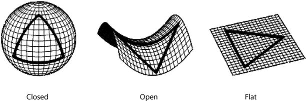
Fig. 4.6
Two-dimensional analogies for the three
possible curvatures of space. In a universe with positive curvature
(K > 0) the sum of the
angles in a triangle is larger than 180∘, in a universe
of negative curvature it is smaller than 180∘, and in a
flat universe the sum of angles is exactly 180∘. Adopted
from J.A. Peacock 1999, Cosmological Physics, Cambridge
University Press
where in the final step we inserted the CMB
temperature; here,  is the reduced
Planck constant. This energy density corresponds to a density
parameter of
is the reduced
Planck constant. This energy density corresponds to a density
parameter of
 As will be explained below, the photons are not the only
contributors to the radiation energy density. In addition, there
are neutrinos from the early cosmic epoch which add to the density
parameter of radiation, which then becomes
As will be explained below, the photons are not the only
contributors to the radiation energy density. In addition, there
are neutrinos from the early cosmic epoch which add to the density
parameter of radiation, which then becomes
 so that today, the energy density of radiation in the Universe can
be neglected when compared to that of matter. However,
(4.24) reveal
that the ratio between matter and radiation density was different
at earlier epochs since ρ
r evolves faster with a than ρ m,
so that today, the energy density of radiation in the Universe can
be neglected when compared to that of matter. However,
(4.24) reveal
that the ratio between matter and radiation density was different
at earlier epochs since ρ
r evolves faster with a than ρ m,
 Thus radiation and dust had the same energy density at an epoch
when the scale factor was
Thus radiation and dust had the same energy density at an epoch
when the scale factor was
 This value of the scale factor and the corresponding epoch in
cosmic history play a very important role in structure evolution in
the Universe, as we will see in Chap. 7.
This value of the scale factor and the corresponding epoch in
cosmic history play a very important role in structure evolution in
the Universe, as we will see in Chap. 7.
is the reduced
Planck constant. This energy density corresponds to a density
parameter of
(4.27)
(4.28)
(4.29)
(4.30)
With  and (4.25), the expansion
equation (4.18) can be written as
and (4.25), the expansion
equation (4.18) can be written as
![$$\displaystyle{ H^{2}(t) = H_{ 0}^{2}\,\left [ \frac{\varOmega _{\mathrm{r}}} {a^{4}(t)} + \frac{\varOmega _{\mathrm{m}}} {a^{3}(t)} - \frac{Kc^{2}} {H_{0}^{2}\,a^{2}(t)} +\varOmega _{\varLambda }\right ]\;. }$$](A129044_2_En_4_Chapter_Equ31.gif) Evaluating this equation at the present epoch, with H(t 0) = H 0 and a(t 0) = 1, yields the value
of the integration constant K,
Evaluating this equation at the present epoch, with H(t 0) = H 0 and a(t 0) = 1, yields the value
of the integration constant K,
 Hence the constant K is
obtained from the density parameters, mainly those of matter and
vacuum since
Hence the constant K is
obtained from the density parameters, mainly those of matter and
vacuum since  ,
and has the dimension of (length)−2. In the context of
GR, K is interpreted as the
curvature scalar of the universe today, or more precisely, the
homogeneous, isotropic three-dimensional space at time t = t 0 has a curvature
K. Depending on the sign of
K, we can distinguish the
following cases:
,
and has the dimension of (length)−2. In the context of
GR, K is interpreted as the
curvature scalar of the universe today, or more precisely, the
homogeneous, isotropic three-dimensional space at time t = t 0 has a curvature
K. Depending on the sign of
K, we can distinguish the
following cases:
and (4.25), the expansion
equation (4.18) can be written as
(4.31)
(4.32)
,
and has the dimension of (length)−2. In the context of
GR, K is interpreted as the
curvature scalar of the universe today, or more precisely, the
homogeneous, isotropic three-dimensional space at time t = t 0 has a curvature
K. Depending on the sign of
K, we can distinguish the
following cases:
-
If K = 0, the three-dimensional space for any fixed time t is Euclidean, i.e., flat.
-
If K < 0, the space is called hyperbolic—the two-dimensional analogy would be the surface of a saddle (see Fig. 4.6).

Hence GR provides a relation between the
curvature of space and the density of the universe. In fact, this
is the central aspect of GR which links the geometry of spacetime
to its matter content. However, Einstein’s theory makes no
statement about the topology of spacetime and, in particular, says
nothing about the topology of the universe.6 If the universe has a simple
topology, it is finite in the case of K > 0, whereas it is infinite if
K ≤ 0. However, in both
cases it has no boundary (compare: the surface of a sphere is a
finite space without boundaries).
![$$\displaystyle{ \fbox{$\begin{array}{rl} \left (\frac{\dot{a}} {a}\right )^{2} & = H^{2}(t) \\ & = H_{0}^{2}\,\left [ \frac{\varOmega _{\mathrm{r}}} {a^{4}(t)} + \frac{\varOmega _{\mathrm{m}}} {a^{3}(t)} + \frac{(1-\varOmega _{\mathrm{m}}-\varOmega _{\varLambda })} {a^{2}(t)} +\varOmega _{\varLambda }\right ] \\ & \equiv H_{0}^{2}E^{2}(t) \end{array} $}\;, }$$](A129044_2_En_4_Chapter_Equ33.gif)

4.3 Consequences of the Friedmann expansion
The cosmic expansion equations imply a number of
immediate consequences, some of which will be discussed next. In
particular, we will first demonstrate that the early Universe must
have evolved out of a very dense and hot state called the
Big Bang. We will then link
the scale factor a to an
observable, the redshift, and explain what the term ‘distance’
means in cosmology.
4.3.1 The necessity of a Big Bang
The terms on the right-hand side
of (4.33) each have a different dependence on
a:
-
For very small a, the first term dominates and the universe is dominated by radiation then.
-
For slightly larger
 , the pressureless matter
(dust) term dominates.
, the pressureless matter
(dust) term dominates. -
If K ≠ 0, the third term, also called the curvature term, can dominate for larger a.
-
For even larger a, the cosmological constant dominates if it is different from zero.
The differential equation (4.33) in general cannot
be solved analytically. However, its numerical solution for
a(t) poses no problems. Nevertheless, we
can analyze the qualitative behavior of the function a(t) and thereby understand the essential
aspects of the expansion history. From the Hubble law, we conclude
that  , i.e., a is currently an increasing function
of time. Equation (4.33) shows that
, i.e., a is currently an increasing function
of time. Equation (4.33) shows that  for all times, unless the
right-hand side of (4.33) vanishes for some value of a: the sign of
for all times, unless the
right-hand side of (4.33) vanishes for some value of a: the sign of  can
only switch when the right-hand side of (4.33) is zero. If
H 2 = 0 for a
value of a > 1, the
expansion will come to a halt and the Universe will recollapse
afterwards. On the other hand, if H 2 = 0 for a value
a = a min with
0 < a
min < 1, then the sign of
can
only switch when the right-hand side of (4.33) is zero. If
H 2 = 0 for a
value of a > 1, the
expansion will come to a halt and the Universe will recollapse
afterwards. On the other hand, if H 2 = 0 for a value
a = a min with
0 < a
min < 1, then the sign of  switches at a
min. At this epoch, a collapsing Universe changes into
an expanding one.
switches at a
min. At this epoch, a collapsing Universe changes into
an expanding one.
, i.e., a is currently an increasing function
of time. Equation (4.33) shows that for all times, unless the
right-hand side of (4.33) vanishes for some value of a: the sign of can
only switch when the right-hand side of (4.33) is zero. If
H 2 = 0 for a
value of a > 1, the
expansion will come to a halt and the Universe will recollapse
afterwards. On the other hand, if H 2 = 0 for a value
a = a min with
0 < a
min < 1, then the sign of
switches at a
min. At this epoch, a collapsing Universe changes into
an expanding one.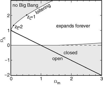
Fig. 4.7
Classification of cosmological models. The
straight solid line
connects flat models (i.e., those without spatial curvature,
 )
and separates open (K < 0) and closed (K > 0) models. The nearly horizontal
curve separates models that will expand forever from those that
will recollapse in the distant future. Models in the upper left
corner have an expansion history where a has never been close to zero and thus
did not experience a Big Bang. In those models, a maximum redshift
for sources exists, which is indicated for two cases. Since we know
that Ω
m > 0. 1, and sources at redshift > 6 have been
observed, these models can be excluded. Adopted from J.A. Peacock
1999, Cosmological Physics,
Cambridge University Press
)
and separates open (K < 0) and closed (K > 0) models. The nearly horizontal
curve separates models that will expand forever from those that
will recollapse in the distant future. Models in the upper left
corner have an expansion history where a has never been close to zero and thus
did not experience a Big Bang. In those models, a maximum redshift
for sources exists, which is indicated for two cases. Since we know
that Ω
m > 0. 1, and sources at redshift > 6 have been
observed, these models can be excluded. Adopted from J.A. Peacock
1999, Cosmological Physics,
Cambridge University PressClassification of
model. Which of these alternatives describes our Universe
depends on the density parameters. We find the following
classification (also see Fig. 4.7 and problem 4.3):
-
If Λ = 0, then H 2 > 0 for all a ≤ 1, whereas the behavior for a > 1 depends on Ω m:
-
if Ω m ≤ 1 (or K ≤ 0, respectively), H 2 > 0 for all a: the universe will expand for all times. This behavior is expected from the Newtonian approach because if K ≤ 0, the kinetic energy in any spherical shell is larger than the modulus of the potential energy, i.e., the expansion velocity exceeds the escape velocity and the expansion will never come to a halt.
-
If Ω m > 1 (K > 0), H 2 will vanish for
 .
The universe will have its maximum expansion when the scale factor
is a max and
will recollapse thereafter. In Newtonian terms, the total energy of
any spherical shell is negative, so that it is gravitationally
bound.
.
The universe will have its maximum expansion when the scale factor
is a max and
will recollapse thereafter. In Newtonian terms, the total energy of
any spherical shell is negative, so that it is gravitationally
bound.
We thus have reobtained the classification discussed before in Sect. 4.2.3, which is valid for Λ = 0, for which the qualitative behavior of the expansion depends only on the sign of K. -
-
In the presence of a cosmological constant Λ > 0, the discussion becomes more complicated; in particular, the geometry of the universe, i.e., the sign of K, is not sufficient to predict the qualitative expansion behavior. For example, there are models with positive curvature (indicated as ‘closed’ in Fig. 4.7) which expand forever. One finds for Λ ≥ 0:
-
If Ω m < 1, the universe will expand for all a > 1.
-
However, for Ω m > 1 the future behavior of a(t) depends on Ω Λ : if Ω Λ is sufficiently small, a value a max exists at which the expansion comes to a halt and reverses. In contrast, if Ω Λ is large enough the universe will expand forever.
-
If Ω Λ < 1, then H 2 > 0 for all a ≤ 1.
-
However, if Ω Λ > 1, it is in principle possible that H 2 = 0 for an a = a min < 1. Such models, in which a minimum value for a existed in the past (so-called bouncing models), can be excluded by observations (see Sect. 4.3.2).
-
With the exception of the last case, which can be
excluded, we come to the conclusion that a must have attained the value
a = 0 at some point in the
past, at least formally. At this instant the ‘size of the Universe’
formally vanished. As a → 0, both matter and radiation
densities diverge so that the density in this state must have been
singular. The epoch at which a = 0 and the evolution away from this
state is called the Big
Bang. It is useful to define this epoch (a = 0) as the origin of time, so that
t is identified with the
age of the Universe, the time since the Big Bang. As we will show,
the predictions of the Big Bang model are in impressive agreement
with observations.
The expansion history for the special case of a
vanishing vacuum energy density is sketched in Fig. 4.8 for three values of
the curvature.
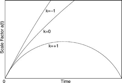
Fig. 4.8
The scale factor a(t) as a function of cosmic time
t for three models with a
vanishing cosmological constant, Ω Λ = 0. Closed models
(K > 0) attain a maximum
expansion and then recollapse. In contrast, open models
(K ≤ 0) expand forever, and
the Einstein–de Sitter model of K = 0 separates these two cases. In all
models, the scale factor tends towards zero in the past; this time
is called the Big Bang and defines the origin of the time
axis
To characterize whether the current expansion of
the Universe is decelerated or accelerated, the deceleration parameter
 is defined where the right-hand side has to be evaluated at
t = t 0. With (4.19)
and (4.33) it follows that
is defined where the right-hand side has to be evaluated at
t = t 0. With (4.19)
and (4.33) it follows that
 If Ω Λ = 0 then q 0 > 0,
  , i.e., the expansion decelerates,
as expected due to gravity. However, if Ω Λ is sufficiently large the
deceleration parameter may become negative, corresponding to an
accelerated expansion of the universe. The reason for this
behavior, which certainly contradicts intuition, is seen in the
vacuum energy. Only a negative pressure can cause an accelerated
expansion—more precisely, as seen from (4.22),
, i.e., the expansion decelerates,
as expected due to gravity. However, if Ω Λ is sufficiently large the
deceleration parameter may become negative, corresponding to an
accelerated expansion of the universe. The reason for this
behavior, which certainly contradicts intuition, is seen in the
vacuum energy. Only a negative pressure can cause an accelerated
expansion—more precisely, as seen from (4.22),  is needed for
  . Indeed, we know today that our
Universe is currently undergoing an accelerated expansion and thus
that the cosmological constant differs significantly from
zero.
. Indeed, we know today that our
Universe is currently undergoing an accelerated expansion and thus
that the cosmological constant differs significantly from
zero.
(4.34)
(4.35)
, i.e., the expansion decelerates,
as expected due to gravity. However, if Ω Λ is sufficiently large the
deceleration parameter may become negative, corresponding to an
accelerated expansion of the universe. The reason for this
behavior, which certainly contradicts intuition, is seen in the
vacuum energy. Only a negative pressure can cause an accelerated
expansion—more precisely, as seen from (4.22), is needed for . Indeed, we know today that our
Universe is currently undergoing an accelerated expansion and thus
that the cosmological constant differs significantly from
zero.Age of the
universe. The age of the universe at a given scale factor
a follows from  .
This relation can be integrated,
.
This relation can be integrated,
![$$\displaystyle\begin{array}{rcl} t(a)& =& \frac{1} {H_{0}}\int _{0}^{a}\,\mathrm{d}x\,\left [x^{-2}\varOmega _{ \mathrm{r}} + x^{-1}\varOmega _{ \mathrm{m}} + (1 -\varOmega _{\mathrm{m}} -\varOmega _{\varLambda })\right. \\ & & \ \left.+x^{2}\varOmega _{ \varLambda }\right ]^{-1/2}\;, {}\end{array}$$](A129044_2_En_4_Chapter_Equ36.gif) where the contribution from radiation for
where the contribution from radiation for  can be neglected because it
is relevant only for very small a and thus only for a very small
fraction of cosmic time. To obtain the current age t 0 of the
universe, (4.36) is calculated for a = 1. For models of vanishing spatial
curvature K = 0 and for
those with Λ = 0,
Fig. 4.9
displays t 0 as
a function of Ω
m.
can be neglected because it
is relevant only for very small a and thus only for a very small
fraction of cosmic time. To obtain the current age t 0 of the
universe, (4.36) is calculated for a = 1. For models of vanishing spatial
curvature K = 0 and for
those with Λ = 0,
Fig. 4.9
displays t 0 as
a function of Ω
m.
.
This relation can be integrated,
(4.36)
can be neglected because it
is relevant only for very small a and thus only for a very small
fraction of cosmic time. To obtain the current age t 0 of the
universe, (4.36) is calculated for a = 1. For models of vanishing spatial
curvature K = 0 and for
those with Λ = 0,
Fig. 4.9
displays t 0 as
a function of Ω
m.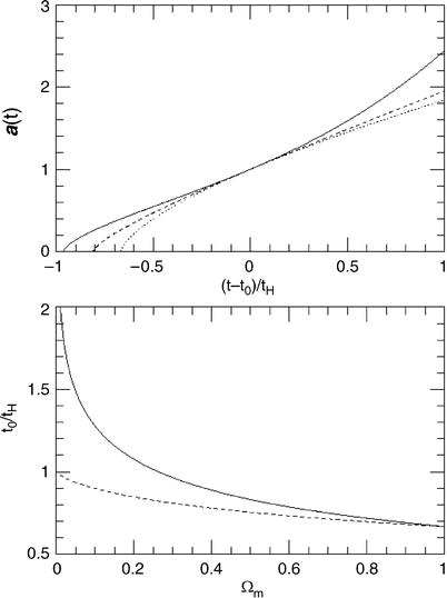
Fig. 4.9
Top
panel: Scale factor a(t) as a function of cosmic time, here
scaled as (t − t 0)H 0, for an Einstein–de
Sitter model (Ω
m = 1, Ω
Λ = 0;
dotted curve), an open
universe (Ω
m = 0. 3, Ω
Λ = 0;
dashed curve), and a flat
universe of low density (Ω
m = 0. 3, Ω
Λ = 0. 7;
solid curve). At the
current epoch, t = t 0 and a = 1. Bottom panel: Age of the universe in
units of the Hubble time  for flat world models
with K = 0 (
for flat world models
with K = 0 ( ;
solid curve) and models
with a vanishing cosmological constant (dashed curve). We see that for a flat
universe with small Ω
m (thus large
;
solid curve) and models
with a vanishing cosmological constant (dashed curve). We see that for a flat
universe with small Ω
m (thus large  ),
t 0 may be
considerably larger than H
0 −1. Credit: M. Bartelmann, MPA
Garching
),
t 0 may be
considerably larger than H
0 −1. Credit: M. Bartelmann, MPA
Garching
for flat world models
with K = 0 (;
solid curve) and models
with a vanishing cosmological constant (dashed curve). We see that for a flat
universe with small Ω
m (thus large ),
t 0 may be
considerably larger than H
0 −1. Credit: M. Bartelmann, MPA
GarchingThe qualitative behavior of the cosmological
models is characterized by the density parameters Ω m and Ω Λ , whereas the Hubble constant
H 0 determines
‘only’ the overall length- or time-scale. One can consider several
special cases for the density parameters:
-
Models without a cosmological constant, Λ = 0. The difficulties in deriving a ‘sensible’ value for Λ from particle physics has in the past often been used as an argument for neglecting the vacuum energy density. However, there are now very strong observational indications that in fact Λ > 0.
-
Models with
 ,
i.e., K = 0. Such flat
models are preferred by the so-called inflationary models, which we
will briefly discuss further below.
,
i.e., K = 0. Such flat
models are preferred by the so-called inflationary models, which we
will briefly discuss further below. -
A special case is the Einstein–de Sitter model, Ω m = 1, Ω Λ = 0. For this model,
 .
. -
For many world models, t 0 is larger than the age of the oldest globular clusters, so they are compatible with this age determination. The Einstein–de Sitter model, however, is compatible with stellar ages only if H 0 is very small, considerably smaller than the value of H 0 derived from the HST Key Project discussed in Sect. 3.9. Hence, this model is ruled out by these observations.
The values of the cosmological parameters are now
quite well known. We list them here for later reference without any
further discussion. Their determination will be described in the
course of this chapter and in Chap. 8. The values are approximately

(4.37)
Early
expansion. In the early phase of the universe, the curvature
term and the vacuum energy density can be neglected in the
expansion equation (4.33), which then simplifies to
 where we used (4.30). In this case, the
relation (4.36) between time and scale factor can be
integrated explicitly to yield
where we used (4.30). In this case, the
relation (4.36) between time and scale factor can be
integrated explicitly to yield
![$$\displaystyle{ t = \frac{2} {3H_{0}\sqrt{\varOmega _{\mathrm{m}}}}\left [a^{3/2}\left (1 -\frac{2a_{\mathrm{eq}}} {a} \right )\sqrt{1 + \frac{a_{\mathrm{eq } } } {a}} + 2a_{\mathrm{eq}}^{3/2}\right ]\;. }$$](A129044_2_En_4_Chapter_Equ38.gif) From this result we can infer that the scale factor behaves at
From this result we can infer that the scale factor behaves at
 for a ≪ a eq and that
  in the matter dominated
era.
in the matter dominated
era.
(4.38)
for a ≪ a eq and that in the matter dominated
era.4.3.2 Redshift
The Hubble law describes a relation between the
redshift, or the radial component of the relative velocity, and the
distance of an object from us. Furthermore, (4.6) specifies that any
observer is experiencing a local Hubble law with an expansion rate
H(t) which depends on the cosmic epoch.
We will now derive a relation between the redshift of a source,
which is directly observable, and the cosmic time t or the scale factor a(t), respectively, at which the source
emitted the light we receive today.
To do this, we consider a light ray that reaches
us today. Along this light ray we imagine fictitious comoving
observers. The light ray is parametrized by the cosmic time
t, and is supposed to have
been emitted by the source at epoch t e. Two comoving observers
along the light ray with separation dr from each other see their relative
motion due to the cosmic expansion according to (4.6), dv = H(t) dr, and they measure it as a redshift of
light,  .
It takes a time
.
It takes a time  for the light to travel
from one observer to the other. Furthermore, from the definition of
the Hubble parameter,
for the light to travel
from one observer to the other. Furthermore, from the definition of
the Hubble parameter,  , we obtain
the relation
, we obtain
the relation  . Combining these
relations, we find
. Combining these
relations, we find
 The relation
  is now
easily integrated since the equation
is now
easily integrated since the equation  obviously has the solution λ = Ca, where C is a constant. That constant is
determined by the wavelength λ obs of the light as
observed today (i.e., at a = 1), so that
obviously has the solution λ = Ca, where C is a constant. That constant is
determined by the wavelength λ obs of the light as
observed today (i.e., at a = 1), so that
 The wavelength at emission was therefore
  .
On the other hand, the redshift z is defined as
.
On the other hand, the redshift z is defined as  .
From this, we finally obtain the relation
.
From this, we finally obtain the relation
 between the observable z
and the scale factor a
which is linked via (4.36) to the cosmic time. The same relation can
also be derived by considering light rays in GR.
between the observable z
and the scale factor a
which is linked via (4.36) to the cosmic time. The same relation can
also be derived by considering light rays in GR.
.
It takes a time for the light to travel
from one observer to the other. Furthermore, from the definition of
the Hubble parameter, , we obtain
the relation . Combining these
relations, we find
(4.39)
is now
easily integrated since the equation
obviously has the solution λ = Ca, where C is a constant. That constant is
determined by the wavelength λ obs of the light as
observed today (i.e., at a = 1), so that
(4.40)
.
On the other hand, the redshift z is defined as .
From this, we finally obtain the relation
(4.41)
The relation between redshift and the scale
factor is of immense importance for cosmology because, for most
sources, redshift is the only distance information that we are able
to measure. If the scale factor is a monotonic function of time,
i.e., if the right-hand side of (4.33) is different from
zero for all a ∈ [0, 1],
then z is also a monotonic
function of t. In this
case, which corresponds to the Universe we happen to live in,
a, t, and z are equally good measures of the
distance of a source from us.
Local Hubble
law. The Hubble law applies for nearby sources:
with (4.8) and v ≈ zc it follows that
 where D is the distance of
a source with redshift z.
This corresponds to a light travel time of
where D is the distance of
a source with redshift z.
This corresponds to a light travel time of  . On the other hand, due to the
definition of the Hubble parameter, we have
. On the other hand, due to the
definition of the Hubble parameter, we have  ,
where a is the scale factor
at time t 0
−Δ t, and we used
a(t 0) = 1 and H(t 0) = H 0. This implies
,
where a is the scale factor
at time t 0
−Δ t, and we used
a(t 0) = 1 and H(t 0) = H 0. This implies
 . Utilizing (4.42), we then find
 ,
or
,
or  ,
which agrees with (4.41) in linear approximation since
,
which agrees with (4.41) in linear approximation since
 . Hence we
conclude that the general relation (4.41) contains the local
Hubble law as a special case.
. Hence we
conclude that the general relation (4.41) contains the local
Hubble law as a special case.
(4.42)
. On the other hand, due to the
definition of the Hubble parameter, we have ,
where a is the scale factor
at time t 0
−Δ t, and we used
a(t 0) = 1 and H(t 0) = H 0. This implies
. Utilizing (4.42), we then find
,
or ,
which agrees with (4.41) in linear approximation since
. Hence we
conclude that the general relation (4.41) contains the local
Hubble law as a special case.Energy density in
radiation. A further consequence of (4.41) is the dependence
of the energy density of radiation on the scale parameter. As
mentioned previously, the number density of photons is  if we assume that photons are
neither created nor destroyed. In other words, the number of
photons in a comoving volume element is conserved. According
to (4.41), the frequency ν of a photon changes due to cosmic
expansion. Since the energy of a photon is ∝ ν,
if we assume that photons are
neither created nor destroyed. In other words, the number of
photons in a comoving volume element is conserved. According
to (4.41), the frequency ν of a photon changes due to cosmic
expansion. Since the energy of a photon is ∝ ν,  , the
energy density of photons decreases, ρ r ∝ n E γ ∝ a −4.
Therefore (4.41) implies (4.24).
, the
energy density of photons decreases, ρ r ∝ n E γ ∝ a −4.
Therefore (4.41) implies (4.24).
if we assume that photons are
neither created nor destroyed. In other words, the number of
photons in a comoving volume element is conserved. According
to (4.41), the frequency ν of a photon changes due to cosmic
expansion. Since the energy of a photon is ∝ ν, , the
energy density of photons decreases, ρ r ∝ n E γ ∝ a −4.
Therefore (4.41) implies (4.24).Cosmic microwave
background. Assuming that, at some time t 1, the universe contained
a blackbody radiation of temperature T 1, we can examine the
evolution of this photon population in time by means of
relation (4.41). We should recall that the Planck
function B
ν (A.13)
specifies the radiation energy of blackbody radiation that passes
through a unit area per unit time, per unit frequency interval, and
per unit solid angle. Using this definition, the number density
dN ν of photons in the frequency
interval between ν and
ν + dν is obtained as
 At a later time t
2 > t
1, the universe has expanded by a factor a(t 2)∕a(t 1). An observer at
t 2 therefore
observes the photons redshifted by a factor
At a later time t
2 > t
1, the universe has expanded by a factor a(t 2)∕a(t 1). An observer at
t 2 therefore
observes the photons redshifted by a factor  , i.e., a photon with
frequency ν at t 1 will then be measured to
have frequency
, i.e., a photon with
frequency ν at t 1 will then be measured to
have frequency  . The original
frequency interval is transformed accordingly as
. The original
frequency interval is transformed accordingly as  .
The number density of photons decreases with the third power of the
scale factor, so that
.
The number density of photons decreases with the third power of the
scale factor, so that  .
Combining these relations, we obtain for the number density
.
Combining these relations, we obtain for the number density
 of photons
in the frequency interval between ν ′ and ν ′ + dν ′
of photons
in the frequency interval between ν ′ and ν ′ + dν ′
 where we used
  in the last step. The
distribution (4.44) has the same form as (4.43) except that the
temperature is reduced by a factor
in the last step. The
distribution (4.44) has the same form as (4.43) except that the
temperature is reduced by a factor  . If a Planck distribution of photons
had been established at an earlier time, it will persist during
cosmic expansion. As we have seen above, the CMB is such a
blackbody radiation, with a current temperature of T 0 = T CMB ≈ 2. 73 K. We will
show in Sect. 4.4 that this radiation originates in the early
phase of the cosmos. Thus it is meaningful to consider the
temperature of the CMB as the ‘temperature of our Universe’ which
is a function of redshift,
. If a Planck distribution of photons
had been established at an earlier time, it will persist during
cosmic expansion. As we have seen above, the CMB is such a
blackbody radiation, with a current temperature of T 0 = T CMB ≈ 2. 73 K. We will
show in Sect. 4.4 that this radiation originates in the early
phase of the cosmos. Thus it is meaningful to consider the
temperature of the CMB as the ‘temperature of our Universe’ which
is a function of redshift,
 i.e., the Universe was hotter in the past than it is today. The
energy density of the Planck spectrum is given
by (4.26), i.e., proportional to T 4, so that ρ r behaves like
i.e., the Universe was hotter in the past than it is today. The
energy density of the Planck spectrum is given
by (4.26), i.e., proportional to T 4, so that ρ r behaves like
 in accordance
with (4.24).7
in accordance
with (4.24).7
(4.43)
, i.e., a photon with
frequency ν at t 1 will then be measured to
have frequency . The original
frequency interval is transformed accordingly as .
The number density of photons decreases with the third power of the
scale factor, so that .
Combining these relations, we obtain for the number density
of photons
in the frequency interval between ν ′ and ν ′ + dν ′
(4.44)
in the last step. The
distribution (4.44) has the same form as (4.43) except that the
temperature is reduced by a factor . If a Planck distribution of photons
had been established at an earlier time, it will persist during
cosmic expansion. As we have seen above, the CMB is such a
blackbody radiation, with a current temperature of T 0 = T CMB ≈ 2. 73 K. We will
show in Sect. 4.4 that this radiation originates in the early
phase of the cosmos. Thus it is meaningful to consider the
temperature of the CMB as the ‘temperature of our Universe’ which
is a function of redshift,
(4.45)
in accordance
with (4.24).7Finally, it should be stressed again
that (4.41) allows all relations to be expressed as
functions of a as well as
of z. For example, the age
of the Universe as a function of z is obtained by replacing the upper
integration limit,  , in (4.36).
, in (4.36).Interpretation of
cosmological redshift. The redshift results from the fact
that during the expansion of the universe, the energy of the
photons decreases in proportion to 1∕a, which is the reason, together with
the decreasing proper number density, that ρ r(a) ∝ a −4. Our considerations in
this section have derived this 1∕a-dependence of the photon
energy.
But maybe this is puzzling anyway—if photons lose
energy during cosmic expansion, then, having in mind the concept of
energy conservation, one might be tempted to ask: Where does this
energy go to?
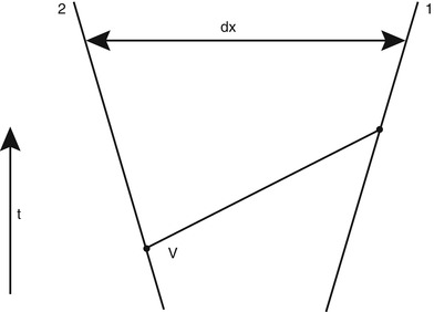
Fig. 4.10
Sketch of two comoving observers with
comoving separation dx, and
a particle with velocity v,
as measured by observer No. 2, moving from the worldline of
observer No. 2 to that of observer No. 1
To answer this question, we start with pointing
out that energy conservation in cosmology is expressed by the
‘first law of thermodynamics’ (4.17), which has as one
of its consequences the 1∕a-behavior of photon energy. Thus,
there is no reason to lose sleep about this issue.
But it may be useful to be more explicit here. We
first point out that ‘the energy’ of a photon, or any other
particle, as such is not defined! To see this, consider two
observers that measure the wavelength of photons; both are at the
same location, but observer No. 2 moves in the direction of the
light source, as seen from observer No. 1. Because of the Doppler
effect, observer No. 2 measures a shorter wavelength than observer
No. 1; thus, the two observers come to different conclusions about
the energy of the photons. It’s not like one of them is right, the
other wrong—the energy of a photon is not an absolute quantity, but
depends on the frame in which it is measured.
We have defined a reference frame in an expanding
universe, that of comoving observers—they are the ones who see the
universe being isotropic around them. When we state that ‘the
photon energy changes as 1∕a’, we implicitly mean that it is the
energy as measured by the comoving observer that changes. As these
comoving observers move relative to each other, as expressed by the
Hubble law, it should not be a surprise that they measure different
frequencies of photons, as explicitly accounted for
in (4.39). Thus, not the properties of the photons
are changing in time, but the state of motion of the observers that
measure the photon energy as they propagate through the
universe.
In fact, one can show that in general the
momentum (as measured by comoving observers!) of a freely moving
particle changes as
 For photons, we have already shown this: since the momentum of a
photon is given by its energy, divided by c, then ν ∝ 1∕a shows the validity
of (4.47). The same is true for other relativistic
particles as well. We can also derive this behavior easily for
non-relativistic particles. Consider a particle of mass
m which crosses the
worldlines of the two neighboring observers 2 and 1 (see
Fig. 4.10).
Let dx be their comoving
separation, then at epoch a
their physical separation is dr = a dx. It takes the particle the time
For photons, we have already shown this: since the momentum of a
photon is given by its energy, divided by c, then ν ∝ 1∕a shows the validity
of (4.47). The same is true for other relativistic
particles as well. We can also derive this behavior easily for
non-relativistic particles. Consider a particle of mass
m which crosses the
worldlines of the two neighboring observers 2 and 1 (see
Fig. 4.10).
Let dx be their comoving
separation, then at epoch a
their physical separation is dr = a dx. It takes the particle the time
 to travel between the
two observers, where v is
the velocity measured by observer No. 2. Observer No. 1 will
measure a velocity v −
dv, since from his
perspective, observer No. 2 is receding from him (this is simply a
Galilean transformation), with a velocity dv = H(a) dr given by the local Hubble law.
Putting this together, there is a momentum change
to travel between the
two observers, where v is
the velocity measured by observer No. 2. Observer No. 1 will
measure a velocity v −
dv, since from his
perspective, observer No. 2 is receding from him (this is simply a
Galilean transformation), with a velocity dv = H(a) dr given by the local Hubble law.
Putting this together, there is a momentum change  of the particle when
measured by the two observers, where
of the particle when
measured by the two observers, where
 where we made use of the definition of the Hubble function. The
resulting equation
where we made use of the definition of the Hubble function. The
resulting equation  has the solution
pa = const.,
i.e., (4.47) holds. For semi-relativistic particles,
the proof of (4.47) can be made with Special Relativity, but
proceeds essentially in the same way.
has the solution
pa = const.,
i.e., (4.47) holds. For semi-relativistic particles,
the proof of (4.47) can be made with Special Relativity, but
proceeds essentially in the same way.
(4.47)
to travel between the
two observers, where v is
the velocity measured by observer No. 2. Observer No. 1 will
measure a velocity v −
dv, since from his
perspective, observer No. 2 is receding from him (this is simply a
Galilean transformation), with a velocity dv = H(a) dr given by the local Hubble law.
Putting this together, there is a momentum change of the particle when
measured by the two observers, where
(4.48)
has the solution
pa = const.,
i.e., (4.47) holds. For semi-relativistic particles,
the proof of (4.47) can be made with Special Relativity, but
proceeds essentially in the same way.The necessity of a
Big Bang. We discussed in Sect. 4.3.1 that the scale
factor must have attained the value a = 0 at some time in the past. One gap
in our argument that inevitably led to the necessity of a Big Bang
still remains, namely the possibility that at some time in the past
 occurred, i.e., that the universe underwent a transition from a
contracting to an expanding state. This is possible only if
Ω Λ > 1 and if the matter
density parameter is sufficiently small (see Fig. 4.7). In this case,
a attained a minimum value
in the past. This minimum value depends on both Ω m and Ω Λ . For instance, for
Ω m > 0. 1,
the value is
occurred, i.e., that the universe underwent a transition from a
contracting to an expanding state. This is possible only if
Ω Λ > 1 and if the matter
density parameter is sufficiently small (see Fig. 4.7). In this case,
a attained a minimum value
in the past. This minimum value depends on both Ω m and Ω Λ . For instance, for
Ω m > 0. 1,
the value is  . But a minimum value
for a implies a maximum
redshift
. But a minimum value
for a implies a maximum
redshift  . However,
since we have observed quasars and galaxies with z > 6 and the density parameter is
known to be Ω
m > 0. 1, such a model without a Big Bang can be
safely excluded.
. However,
since we have observed quasars and galaxies with z > 6 and the density parameter is
known to be Ω
m > 0. 1, such a model without a Big Bang can be
safely excluded.
occurred, i.e., that the universe underwent a transition from a
contracting to an expanding state. This is possible only if
Ω Λ > 1 and if the matter
density parameter is sufficiently small (see Fig. 4.7). In this case,
a attained a minimum value
in the past. This minimum value depends on both Ω m and Ω Λ . For instance, for
Ω m > 0. 1,
the value is . But a minimum value
for a implies a maximum
redshift . However,
since we have observed quasars and galaxies with z > 6 and the density parameter is
known to be Ω
m > 0. 1, such a model without a Big Bang can be
safely excluded.4.3.3 Distances in cosmology
In the previous sections, different distance
measures were discussed. Because of the monotonic behavior of the
corresponding functions, each of a, t, and z provide the means to sort objects
according to their distance. An object at higher redshift
z 2 is more
distant than one at z
1 < z
2 such that light from a source at z 2 may become absorbed by
gas in an object at redshift z 1, but not vice versa. The
object at redshift z
1 is located between us and the object at z 2. The more distant a
source is from us, the longer the light takes to reach us, the
earlier it was emitted, the smaller a was at emission, and the larger
z is. Since z is the only observable of these
parameters, distances in extragalactic astronomy are nearly always
expressed in terms of redshift.
But how can a redshift be translated into a
distance that has the dimension of a length? Or, phrasing this
question differently, how many Megaparsecs away from us is a source
with redshift z = 2? The
corresponding answer is more complicated than the question
suggests. For very small redshifts, the local Hubble
relation (4.42) may be used, but this is valid only for
z ≪ 1.
In a static
Euclidean space, the separation between two points is
unambiguously defined, and several prescriptions exist for
measuring a distance. We will give two examples here. A sphere of
radius R situated at
distance D subtends a solid
angle of  on our sky. If the radius
is known, D can be measured
using this relation. As a second example, we consider a source of
luminosity L at distance
D which then has a measured
flux
on our sky. If the radius
is known, D can be measured
using this relation. As a second example, we consider a source of
luminosity L at distance
D which then has a measured
flux  . Again, if the luminosity is
known, the distance can be computed from the observed flux. If we
use these two methods to determine, for example, the distance to
the Sun, we would of course obtain identical results for the
distance (within the range of accuracy), since these two
prescriptions for distance measurements are defined to yield equal
results.
. Again, if the luminosity is
known, the distance can be computed from the observed flux. If we
use these two methods to determine, for example, the distance to
the Sun, we would of course obtain identical results for the
distance (within the range of accuracy), since these two
prescriptions for distance measurements are defined to yield equal
results.
on our sky. If the radius
is known, D can be measured
using this relation. As a second example, we consider a source of
luminosity L at distance
D which then has a measured
flux . Again, if the luminosity is
known, the distance can be computed from the observed flux. If we
use these two methods to determine, for example, the distance to
the Sun, we would of course obtain identical results for the
distance (within the range of accuracy), since these two
prescriptions for distance measurements are defined to yield equal
results.In a non-Euclidean or expanding/contracting
space-time like, for instance, our Universe this is no longer the
case. The equivalence of different distance measures is only
ensured in Euclidean space, and we have no reason to expect this
equivalence to also hold in a curved spacetime. In cosmology, the
same measuring prescriptions as in Euclidean space are used for
defining distances, but the different definitions lead to different
results. The two most important definitions of distance are:
-
Angular-diameter distance: As above, we consider a source of radius R observed to cover a solid angle ω. The angular-diameter distance is defined as
 (4.49)
 -
Luminosity distance: We consider a source with bolometric luminosity L and flux S and define its luminosity distance as
 (4.50)
These two distances agree locally, i.e., for
z ≪ 1; on small scales, the
curvature of spacetime is not noticeable. In addition, they are
unique functions of
redshift. They can be computed explicitly. However, to do this some
tools of GR are required. Since we have not discussed GR in this
book, these tools are not available to us here. The
distance-redshift relations depend on the cosmological parameters;
Fig. 4.11
shows the angular-diameter distance for different models. For
Λ = 0, the famous Mattig
relation applies,
![$$\displaystyle\begin{array}{rcl} D_{\mathrm{A}}(z)& =& \frac{c} {H_{0}}\, \frac{2} {\varOmega _{\mathrm{m}}^{2}\,(1 + z)^{2}} \\ & & \times \left [\varOmega _{\mathrm{m}}z + (\varOmega _{\mathrm{m}} - 2)\left (\sqrt{1 +\varOmega _{\mathrm{m} } z} - 1\right )\right ]\;.{}\end{array}$$](A129044_2_En_4_Chapter_Equ51.gif)
(4.51)
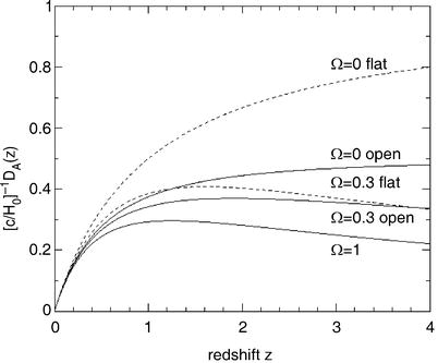
Fig. 4.11
Angular-diameter distance vs. redshift for
different cosmological models. Solid curves display models with no
vacuum energy; dashed
curves show flat models with  .
In both cases, results are plotted for Ω m = 1, 0.3, and 0. Adopted
from J.A. Peacock 1999, Cosmological Physics, Cambridge
University Press
.
In both cases, results are plotted for Ω m = 1, 0.3, and 0. Adopted
from J.A. Peacock 1999, Cosmological Physics, Cambridge
University Press
.
In both cases, results are plotted for Ω m = 1, 0.3, and 0. Adopted
from J.A. Peacock 1999, Cosmological Physics, Cambridge
University PressIn particular, D A is not necessarily a
monotonic function of z. To
better comprehend this, we consider the geometry on the surface of
a sphere. Two great circles on Earth are supposed to intersect at
the North Pole enclosing an angle  —they are therefore meridians. The
separation L between these
two great circles, i.e., the length of the connecting line
perpendicular to both great circles, can be determined as a
function of the distance D
from the North Pole, which is measured as the distance along one of
the two great circles. If θ
is the geographical latitude (
—they are therefore meridians. The
separation L between these
two great circles, i.e., the length of the connecting line
perpendicular to both great circles, can be determined as a
function of the distance D
from the North Pole, which is measured as the distance along one of
the two great circles. If θ
is the geographical latitude ( at the North Pole,
  at the South Pole),
  is found, where
R is the radius of the
Earth. L vanishes at the
North Pole, attains its maximum at the equator (where θ = 0), and vanishes again at the South
Pole; this is because both meridians intersect there again.
Furthermore,
is found, where
R is the radius of the
Earth. L vanishes at the
North Pole, attains its maximum at the equator (where θ = 0), and vanishes again at the South
Pole; this is because both meridians intersect there again.
Furthermore,  , e.g., the distance to the
equator
, e.g., the distance to the
equator  is a quarter of the Earth’s circumference. Solving the last
relation for θ, the
distance is then given by
is a quarter of the Earth’s circumference. Solving the last
relation for θ, the
distance is then given by  .
For the angular-diameter distance on the Earth’s surface, we define
.
For the angular-diameter distance on the Earth’s surface, we define
 , in
analogy to the definition (4.49). For values of D that are considerably smaller than
the curvature radius R of
the sphere, we therefore obtain that D A ≈ D, whereas for larger D, D A deviates considerably
from D. In particular,
D A is not a
monotonic function of D,
rather it has a maximum at
, in
analogy to the definition (4.49). For values of D that are considerably smaller than
the curvature radius R of
the sphere, we therefore obtain that D A ≈ D, whereas for larger D, D A deviates considerably
from D. In particular,
D A is not a
monotonic function of D,
rather it has a maximum at  and then decreases for larger
D.
and then decreases for larger
D.
—they are therefore meridians. The
separation L between these
two great circles, i.e., the length of the connecting line
perpendicular to both great circles, can be determined as a
function of the distance D
from the North Pole, which is measured as the distance along one of
the two great circles. If θ
is the geographical latitude ( at the North Pole, at the South Pole), is found, where
R is the radius of the
Earth. L vanishes at the
North Pole, attains its maximum at the equator (where θ = 0), and vanishes again at the South
Pole; this is because both meridians intersect there again.
Furthermore, , e.g., the distance to the
equator
is a quarter of the Earth’s circumference. Solving the last
relation for θ, the
distance is then given by .
For the angular-diameter distance on the Earth’s surface, we define
, in
analogy to the definition (4.49). For values of D that are considerably smaller than
the curvature radius R of
the sphere, we therefore obtain that D A ≈ D, whereas for larger D, D A deviates considerably
from D. In particular,
D A is not a
monotonic function of D,
rather it has a maximum at and then decreases for larger
D.There exists a general relation between
angular-diameter distance and luminosity distance,
 The reader might now ask which of these distances is the
correct one? Well, this
question does not make sense since there is no unique definition of
the distance in a curved
spacetime like our Universe. Instead, the aforementioned
measurement prescriptions must be used. The choice of a distance
definition depends on the desired application of this distance. For
example, if we want to compute the linear diameter of a source with
observed angular diameter, the angular-diameter distance must be
employed because it is defined just in this way. On the other hand,
to derive the luminosity of a source from its redshift and observed
flux, the luminosity distance needs to be applied. Due to the
definition of the angular-diameter distance (length/angular
diameter), those are the relevant distances that appear in the
gravitational lens equation (3.63).
A statement that a source is located “at a distance of 7 billion
light years” away from us is meaningless unless it is mentioned
which type of distance is meant. Again, in the low-redshift
Universe (z ≪ 1), the
differences between different distance definitions are very small,
and thus it is meaningful
to state, for example, that the Coma cluster of galaxies lies at a
distance of ∼ 90 Mpc.
The reader might now ask which of these distances is the
correct one? Well, this
question does not make sense since there is no unique definition of
the distance in a curved
spacetime like our Universe. Instead, the aforementioned
measurement prescriptions must be used. The choice of a distance
definition depends on the desired application of this distance. For
example, if we want to compute the linear diameter of a source with
observed angular diameter, the angular-diameter distance must be
employed because it is defined just in this way. On the other hand,
to derive the luminosity of a source from its redshift and observed
flux, the luminosity distance needs to be applied. Due to the
definition of the angular-diameter distance (length/angular
diameter), those are the relevant distances that appear in the
gravitational lens equation (3.63).
A statement that a source is located “at a distance of 7 billion
light years” away from us is meaningless unless it is mentioned
which type of distance is meant. Again, in the low-redshift
Universe (z ≪ 1), the
differences between different distance definitions are very small,
and thus it is meaningful
to state, for example, that the Coma cluster of galaxies lies at a
distance of ∼ 90 Mpc.
(4.52)
In Fig. 4.12 a Hubble diagram extending to high
redshifts is shown, where the brightest galaxies in clusters of
galaxies have been used as approximate standard candles. With an
assumed constant intrinsic luminosity for these galaxies, the
apparent magnitude is a measure of their distance, where the
luminosity distance D
L(z) must be
applied to compute the flux as a function of redshift.
Fig. 4.12
A modern Hubble diagram: for several
clusters of galaxies, the K-band magnitude of the brightest cluster
galaxy is plotted versus the escape velocity, measured as redshift
 (symbols). If these galaxies all had the
same luminosity, the apparent magnitude would be a measure of
distance. For low redshifts, the curves follow the linear Hubble
law (4.9), with z ≈ v∕c, whereas for higher redshifts
modifications to this law are necessary. The solid curve corresponds to a constant
galaxy luminosity at all redshifts, whereas the two other
curves take evolutionary
effects of the luminosity into account according to models of
population synthesis (Sect. 3.5). Two different epochs of star
formation were assumed for these galaxies. The diagram is based on
a cosmological model with a deceleration parameter of q 0 = 0 [see (4.35)]. Source: A.
Aragon-Salamanca et al. 1998, The
K-band Hubble diagram for the brightest cluster galaxies: a test of
hierarchical galaxy formation models, MNRAS 297, 427,
p. 429, Fig. 1. Reproduced by permission of Oxford University Press
on behalf of the Royal Astronomical Society
(symbols). If these galaxies all had the
same luminosity, the apparent magnitude would be a measure of
distance. For low redshifts, the curves follow the linear Hubble
law (4.9), with z ≈ v∕c, whereas for higher redshifts
modifications to this law are necessary. The solid curve corresponds to a constant
galaxy luminosity at all redshifts, whereas the two other
curves take evolutionary
effects of the luminosity into account according to models of
population synthesis (Sect. 3.5). Two different epochs of star
formation were assumed for these galaxies. The diagram is based on
a cosmological model with a deceleration parameter of q 0 = 0 [see (4.35)]. Source: A.
Aragon-Salamanca et al. 1998, The
K-band Hubble diagram for the brightest cluster galaxies: a test of
hierarchical galaxy formation models, MNRAS 297, 427,
p. 429, Fig. 1. Reproduced by permission of Oxford University Press
on behalf of the Royal Astronomical SocietyWe compile several expressions that are required
to compute distances in general Friedmann–Lemaître models (see also
problem 4.6).
To do this, we need to define the function
 where K is the curvature
scalar (4.32). The comoving radial distance
x of a source at redshift
z can be computed using
where K is the curvature
scalar (4.32). The comoving radial distance
x of a source at redshift
z can be computed using
 .
Hence with (4.33)
.
Hence with (4.33)
 The angular-diameter distance is then given as
![$$\displaystyle{ D_{\mathrm{A}}(z) = \frac{1} {1 + z}\,f_{K}\left [x(z)\right ]\;, }$$](A129044_2_En_4_Chapter_Equ54.gif) and thus can be computed for all redshifts and cosmological
parameters by (in general numerical) integration
of (4.53). The luminosity distance then follows
from (4.52). The angular-diameter distance of a
source at redshift z
2, as measured by an observer at redshift z 1 < z 2, reads
and thus can be computed for all redshifts and cosmological
parameters by (in general numerical) integration
of (4.53). The luminosity distance then follows
from (4.52). The angular-diameter distance of a
source at redshift z
2, as measured by an observer at redshift z 1 < z 2, reads
![$$\displaystyle{ D_{\mathrm{A}}(z_{1},z_{2}) = \frac{1} {1 + z_{2}}\,f_{K}\left [x(z_{2}) - x(z_{1})\right ]\;. }$$](A129044_2_En_4_Chapter_Equ55.gif) This is the distance that is required in equations of gravitational
lens theory for D
ds. In particular,
This is the distance that is required in equations of gravitational
lens theory for D
ds. In particular,  .
.
.
Hence with (4.33)
(4.53)
(4.54)
(4.55)
.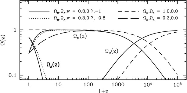
Fig. 4.13
The ratio of the density of the different
components in the universe to the critical density  , as a
function of redshift, for four different cosmological models: the
solid curves correspond to
the model which is presumably the one we live in, the short-dashed curves correspond to an
Einstein–de Sitter model, and the long-dashed curves show a low density
universe without dark energy. Finally, the dotted curve corresponds to a case with
a different model for the dark energy. In all cases, radiation
dominates the energy density of the universe at early times, i.e.,
at high redshifts, whereas for z below ∼ 104 the universe
becomes matter dominated. Only at redshift below ∼ 2 does dark
energy contribute significantly to the energy budget, but then
quickly starts to dominate. Source: M. Voit 2004, Tracing cosmic evolution with clusters of
galaxies, astro-ph/0410173, Fig. 2. Reproduced with
permission of the author
, as a
function of redshift, for four different cosmological models: the
solid curves correspond to
the model which is presumably the one we live in, the short-dashed curves correspond to an
Einstein–de Sitter model, and the long-dashed curves show a low density
universe without dark energy. Finally, the dotted curve corresponds to a case with
a different model for the dark energy. In all cases, radiation
dominates the energy density of the universe at early times, i.e.,
at high redshifts, whereas for z below ∼ 104 the universe
becomes matter dominated. Only at redshift below ∼ 2 does dark
energy contribute significantly to the energy budget, but then
quickly starts to dominate. Source: M. Voit 2004, Tracing cosmic evolution with clusters of
galaxies, astro-ph/0410173, Fig. 2. Reproduced with
permission of the authorSometimes, the look-back time is used as another
quantity characterizing the ‘distance’ of a source. It is defined
as the time the light traveled from a source at redshift
z to us, and can be
calculated in analogy to (4.36), with the lower and upper limit of
integration being  and 1, respectively.
and 1, respectively.4.3.4 Special case: The Einstein–de Sitter model
As a final note in this section, we will briefly
examine one particular cosmological model more closely, namely the
model with Ω
Λ = 0 and
vanishing curvature, K = 0,
and hence Ω
m = 1. We disregard the radiation component, which
contributes to the expansion only at very early times and thus for
very small a. For a long
time, this Einstein–de Sitter (EdS) model was the preferred model
among cosmologists because inflation (see Sect. 4.5.3) predicts
K = 0 and because a finite
value for the cosmological constant was considered ‘unnatural’. In
fact, as late as the mid-1990s, this model was termed the ‘standard
model’. In the meantime we have learned that Λ ≠ 0; thus we are not living in an EdS
universe. But there is at least one good reason to examine this
model a bit more, since the expansion equations become much simpler
for these parameters and we can formulate simple explicit
expressions for the quantities introduced above. These then yield
estimates which for other model parameter values are only possible
by means of numerical integration.
The resulting expansion equation  is easily solved by
making the ansatz a = (Ct) β which, when inserted into the
equation, yields the solution
is easily solved by
making the ansatz a = (Ct) β which, when inserted into the
equation, yields the solution
 Setting a = 1, we obtain
the age of the Universe,
Setting a = 1, we obtain
the age of the Universe,  . The same result also follows
immediately from (4.36) if the parameters of an EdS model are
inserted there. Using
. The same result also follows
immediately from (4.36) if the parameters of an EdS model are
inserted there. Using  results in an age of about 10 Gyr, which is slightly too low to be
compatible with the age of the oldest star clusters. The
angular-diameter distance (4.49) in an EdS universe is obtained by
considering the Mattig relation (4.41) for the case
Ω m = 1:
results in an age of about 10 Gyr, which is slightly too low to be
compatible with the age of the oldest star clusters. The
angular-diameter distance (4.49) in an EdS universe is obtained by
considering the Mattig relation (4.41) for the case
Ω m = 1:
 where we used (4.52) to obtain the second relation from the
first.
where we used (4.52) to obtain the second relation from the
first.
is easily solved by
making the ansatz a = (Ct) β which, when inserted into the
equation, yields the solution
(4.56)
. The same result also follows
immediately from (4.36) if the parameters of an EdS model are
inserted there. Using
results in an age of about 10 Gyr, which is slightly too low to be
compatible with the age of the oldest star clusters. The
angular-diameter distance (4.49) in an EdS universe is obtained by
considering the Mattig relation (4.41) for the case
Ω m = 1:
(4.57)
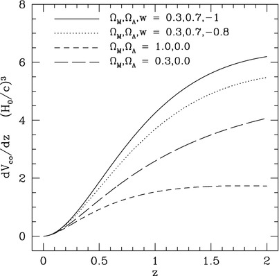
Fig. 4.14
The comoving volume of spherical shells per
unit redshift interval, scaled by (c∕H 0)3, for the
same cosmological models as shown in Fig. 4.13. Obviously, the
transformation of a redshift interval into a volume element is a
strong function of the density parameters; the volume is smallest
for the Einstein–de Sitter model, and largest for the flat,
low-density universe. Source: M. Voit 2004, Tracing cosmic evolution with clusters of
galaxies, astro-ph/0410173, Fig. 3. Reproduced with
permission of the author
4.3.5 Summary
We shall summarize the most important points of
the two preceding lengthy sections:
-
Observations are compatible with the fact that the Universe around us is isotropic and homogeneous on large scales. The cosmological principle postulates this homogeneity and isotropy of the Universe.
-
General Relativity allows homogeneous and isotropic world models, the Friedmann–Lemaître models. In the language of GR, the cosmological principle reads as follows: “A family of solutions of Einstein’s field equations exists such that a set of comoving observers see the same history of the universe; for each of them, the universe appears isotropic.”
-
The shape of these Friedmann–Lemaître world models is characterized by the density parameter Ω m and by the cosmological constant Ω Λ , the size by the Hubble constant H 0. The cosmological parameters determine the expansion rate of the universe as a function of time.
-
The scale factor a(t) of the universe is a monotonically increasing function from the beginning of the universe until now; at earlier times the universe was smaller, denser, and hotter. There must have been an instant when a → 0, which is called the Big Bang. The future of the expansion depends on Ω m and Ω Λ .
-
The expansion of the universe causes a redshift of photons. The more distant a source is from us, the more its photons are redshifted.
-
The relative contribution of radiation, matter and vacuum energy density changes over cosmic time, with radiation dominating in the first phase of the universe, changing to a matter-dominated universe, to become dark-energy dominated at late times, provided Ω Λ > 0 (see Fig. 4.13).
-
‘Distance’ in cosmology does not have a unique meaning. Depending on whether one relates fluxes to luminosity, or length scales with angular sizes, one needs to use different definitions of distances. The distance-redshift relations depend on the values of the cosmological parameters—they all scale with the Hubble length c∕H 0, and depend on the density parameters. Accordingly, the volume of a spherical shell with given thickness in redshift also depends on the density parameters—which is important when source counts are used to infer number density of sources (see Fig. 4.14).
At http://www.astro.ucla.edu/~wright/CosmoCalc.html
the reader can find an online calculator for distances, ages,
lookback-times etc. as a function of redshift, for different
cosmological parameters.
4.4 Thermal history of the Universe
Since T ∝ (1 + z) our Universe was hotter at earlier
times. For example, at a redshift of z = 1100 the temperature (of the CMB)
was about T ∼ 3000 K. And
at an even higher redshift, z = 109, it was T ∼ 3 × 10⁹ K, hotter than
in a stellar interior. Thus we might expect energetic processes
like nuclear fusion to have taken place in the early
Universe.
In this section we shall describe the essential
processes in the early universe. To do so we will assume that the
laws of physics have not changed over time. This assumption is by
no means trivial—we have no guarantee whatsoever that the cross
sections in nuclear physics were the same 13 billion years ago as
they are today. But if they have changed in the course of time the
only chance of detecting this is through cosmology. Based on this
assumption of time-invariant physical laws, we will study the
consequences of the Big Bang model developed in the previous
section and then compare them with observations. Only this
comparison can serve as a test of the success of the model. A few
comments should serve as preparation for the discussion in this
section.
1.
Temperature and energy may be converted into each
other since k B
T has the dimension of
energy. We use the electron volt (eV) to measure temperatures and
energies, with the conversion  .
.
.2.
Elementary particle physics is very well
understood for energies below ∼ 100 GeV. For much higher energies
our understanding of physics is a lot less certain. Therefore, we
will begin the consideration of the thermal history of the cosmos
at energies well below this scale.
3.
Statistical physics and thermodynamics of
elementary particles are described by quantum mechanics. A
distinction has to be made between bosons, which are particles of integer
spin (like the photon), and fermions, particles of half-integer
spin (like, for instance, electrons, protons, neutrinos, and their
anti-particles).
4.
If particles are in thermodynamical and chemical
equilibrium, their number density and their energy distribution are
specified solely by the temperature—e.g., the Planck
distribution (A.13), and thus the energy density of the
radiation (4.26), is a function of T only.
The necessary condition for establishing chemical
equilibrium is the possibility for particles to be created and
destroyed, such as in e+-e−-pair production
andannihilation.
4.4.1 The Standard Model of particle physics
Before discussing the events in the early history
of the Universe in more detail, it is useful to briefly summarize
what we know about particle physics. Since about the 1970s, the
Standard Model has been in place; it describes the elementary
particles and their interactions—except for gravity.

Fig. 4.15
The particles in the Standard Model: The
six quarks (violet) and six
leptons (green) are
organized in three families; the four gauge bosons are shown in
red. The numbers in each box indicate particle
mass, charge (in units of the elementary charge) and spin. All
particles have an antiparticle, except the photon and the Z-boson,
which are their own antiparticles. Not shown in the diagram is the
recently found Higgs particle. Source: Wikipedia
Particle
contents. According to this model, matter is composed of
fermions, particles with half-integer spin, which obey the Pauli
exclusion principle. The fermions are further divided into leptons,
such as the electron and the electron neutrino, and quarks, such as
the up and down quark. Figure 4.15 provides an overview on the particles of
the Standard Model, together with information on their mass, charge
and spin. All of the particles have anti-particles; for example,
the positron is the anti-particle of the electron, its charge is
minus the electron’s charge; some of the particles are their own
anti-particle, such as the photon. The quarks, particles with the
strange property that their charge is not a multiple of the
elementary charge, but thirds of it, form bound states, such as the
proton and the neutron, being composed of three quarks each. In
fact, according to the Standard Model, quarks do not occur isolated
in nature, but are only found in compound systems of hadrons, such
as the nucleons, or mesons, such as the pions. According to the
model, the former consist of three quarks, the latter of a
quark-antiquark system. Protons and neutrons are composed and up
and down quarks, the lightest quarks. The electron, the electron
neutrino, and the up and down quarks form the so-called first
family of particles (see Fig. 4.15).
Except for the electron, there are two more
charged leptons, the muon and the tau, which were discovered in
1936 and 1975, respectively. Both of these leptons are much heavier
than the electron, and they are unstable: the muon decays into an
electron and two neutrinos, whereas the tau can either decay into a
muon or an electron, again accompanied with two neutrinos. However,
these two charged leptons show properties very similar to those of
the electron. For both of them, there is an associated neutrino,
the μ-neutrino
(ν μ ) and the τ-neutrino (ν τ ). Neutrinos are much more
difficult to detect than the charged leptons, since they only
interact weakly with matter. Therefore, they were directly detected
only in 1956 (ν
e), 1962 (ν
μ ) and 2000
(ν τ )—note that the discovery of
the tau-neutrino occurred well after the Standard Model had been
well established and presents one of its successes.
Particle accelerators with ever increasing
energies produced heavier particles. Among them were also particles
which could not be described as composite particles consisting of
up and down quarks only, but their understanding implied the
presence of additional quarks. By 1970, the strange and charm
quarks were thereby indirectly discovered. Together with the muon
and its neutrino, these two new quarks form the second family of
elementary particles. With the discovery of the tau, two more
quarks were predicted, to form the third family—the bottom and top
quark were indeed discovered in 1977 and 1995, again as bound
states forming heavier compound particles.
Interactions;
gauge bosons. According to the Standard Model, interactions
between particles occur through the exchange of bosons. The carrier
of the electromagnetic force is the photon. The exchange particles
for the strong force between quarks is the gluon. Like the photon,
it is electrically neutral, but unlike the photon, it carries a new
property called color. As for the quarks, an isolated gluon has not
been observed yet; nevertheless, its existence was indirectly
verified in particle decays in 1979. The strong interaction between
quarks transmitted by gluons is described by the theory of Quantum
Chromodynamics (QCD), which is the strong interaction part of the
Standard Model.
All leptons are subject to weak interactions; the
Standard Model postulates the existence of two exchange bosons, the
charged W-boson and the electrically neutral Z-boson. Their
discovery had to await sufficiently powerful accelerators, but both
were finally found in 1983, a beautiful and impressive confirmation
of the Standard Model. The Standard Model predicts that
electromagnetic and weak interactions are unified to the
electroweak interaction. However, at low energies these two
interactions appear to be quite different. The explanation for this
difference is that the W- and Z-boson are very massive, whereas the
photon is massless. Thus, at energy scales below the Z-boson mass,
weak interactions are considerably weaker than electromagnetic
ones.
The Higgs
mechanism. According to the Standard Model as outlined so
far, all particles are intrinsically massless. Obviously, this is
not the case; for example, the electron, the muon and the tau have
a finite rest mass. One finds that the quarks have a finite rest
mass as well. As an aside, we note that the mass of a nucleon is
much higher than the sum of the masses of its three constituent
quarks; most of the nucleon mass stems from the strong interactions
transmitted by the gluons.
A mechanism for particles to obtain a finite rest
mass was proposed in the 1960s, and this so-called Higgs-mechanism
for symmetry breaking has been widely accepted and became part of
the Standard Model. It is responsible for the large masses of the W
and Z bosons, and thus for the different appearance of electroweak
interactions as weak and electromagnetic ones at low energies. This
Higgs mechanism implies the existence of an additional particle,
called the Higgs particle. The search for this Higgs particle was
one of the main drivers for building the most complex machine ever
made by mankind—the Large Hadron Collider at CERN. It can generate
sufficiently high energies for the Higgs particle to be generated
and discovered. Indeed, in the summer of 2013, scientists from two
different collaborations announced the discovery of a new
elementary particle, which after a short period was verified as
being the long-sought Higgs particle—a spectacular success! With
that, the final missing piece of the Standard Model was found. The
Nobel Prize in physics 2013 for F. Englert and P. Higgs for the
theoretical development of this mechanism acknowledges also the
importance of this discovery.
4.4.2 Expansion in the radiation-dominated phase
As mentioned above (4.30), the energy density
of radiation dominates in the early universe, at redshifts
z ≫ z eq where
 The radiation density behaves like
  , where the
constant of proportionality depends on the number of species of
relativistic particles (these are the ones for which
, where the
constant of proportionality depends on the number of species of
relativistic particles (these are the ones for which  ). Since T ∝ 1∕a and thus ρ r ∝ a −4, radiation then
dominates in the expansion equation (4.18). The latter can be
solved by a power law, a(t) ∝ t β , which after insertion into
the expansion equation yields
). Since T ∝ 1∕a and thus ρ r ∝ a −4, radiation then
dominates in the expansion equation (4.18). The latter can be
solved by a power law, a(t) ∝ t β , which after insertion into
the expansion equation yields  and thus
 where the constant of proportionality depends again on the number
of relativistic particle species. Since the latter is known from
particle physics, assuming thermodynamical equilibrium, the time
dependence of the early expansion is uniquely specified
by (4.59). This is reasonable because for early
times neither the curvature term nor the cosmological constant
contribute significantly to the expansion dynamics.
where the constant of proportionality depends again on the number
of relativistic particle species. Since the latter is known from
particle physics, assuming thermodynamical equilibrium, the time
dependence of the early expansion is uniquely specified
by (4.59). This is reasonable because for early
times neither the curvature term nor the cosmological constant
contribute significantly to the expansion dynamics.
(4.58)
, where the
constant of proportionality depends on the number of species of
relativistic particles (these are the ones for which ). Since T ∝ 1∕a and thus ρ r ∝ a −4, radiation then
dominates in the expansion equation (4.18). The latter can be
solved by a power law, a(t) ∝ t β , which after insertion into
the expansion equation yields and thus
(4.59)
4.4.3 Decoupling of neutrinos
We start our consideration of the universe at a
temperature of T ≈ 1012 K which corresponds
to ∼ 100 MeV. This energy can be compared to the rest mass of
various particles:
proton,  ,
,
,neutron,  ,
,
,electron,  ,
,
,muon,  .
.
.Protons and neutrons (i.e., the baryons) are too
heavy to be produced at the temperature considered. Thus all
baryons that exist today must have been present already at this
early time. Also, the production of muon pairs, according to the
reaction  , is
not efficient because the temperature, and thus the typical photon
energy, is not sufficiently high. Hence, at the temperature
considered the following relativistic particle species are present:
electrons and positrons, photons and neutrinos. These species
contribute to the radiation density ρ r. The mass of the
neutrinos is not accurately known, though we recently learned that
they have a small but finite rest mass. As will be explained in
Sect. 8.7, cosmology allows us to obtain a
very strict limit on the neutrino mass, which is currently below
1 eV. For the purpose of this discussion they may thus be
considered as massless.
, is
not efficient because the temperature, and thus the typical photon
energy, is not sufficiently high. Hence, at the temperature
considered the following relativistic particle species are present:
electrons and positrons, photons and neutrinos. These species
contribute to the radiation density ρ r. The mass of the
neutrinos is not accurately known, though we recently learned that
they have a small but finite rest mass. As will be explained in
Sect. 8.7, cosmology allows us to obtain a
very strict limit on the neutrino mass, which is currently below
1 eV. For the purpose of this discussion they may thus be
considered as massless.In addition to relativistic particles,
non-relativistic particles also exist. These are the protons and
neutrons, and probably also the constituents of dark matter. We
assume that the latter consists of weakly interacting massive
particles ( WIMPs), with rest mass larger than ∼ 100 GeV because up
to these energies no WIMP candidates have been found in terrestrial
particle accelerator laboratories. With this assumption, WIMPs are
non-relativistic at the energies considered. Thus, like the
baryons, they virtually do not contribute to the energy density in
the early universe.
Apart from the WIMPs, all the aforementioned
particle species are in equilibrium, e.g., by the following
reactions:
 :
Compton scattering,
:
Compton scattering, :
pair-production and annihilation,
:
pair-production and annihilation, :
neutrino-antineutrino-scattering,
:
neutrino-antineutrino-scattering, :
neutrino-electron scattering,
:
neutrino-electron scattering, :
Bremsstrahlung.
:
Bremsstrahlung.Reactions involving baryons will be discussed
later. The energy density at this epoch is8
 which yields—see (4.59)—
 Hence, about one second after the Big Bang the temperature of the
Universe was about 1010 K. For the particles to maintain
equilibrium, the reactions above have to occur at a sufficient
rate. The equilibrium state, specified by the temperature,
continuously changes due to the expansion of the Universe, so that
the particle distribution needs to continually adjust to this
changing equilibrium. This is possible only if the mean time
between two reactions is much shorter than the time-scale on which
equilibrium conditions change. The latter is given by the
expansion. This means that the reaction rates (the number of
reactions per particle per unit time) must be larger than the
cosmic expansion rate H(t) in order for the particles to
maintain equilibrium.
Hence, about one second after the Big Bang the temperature of the
Universe was about 1010 K. For the particles to maintain
equilibrium, the reactions above have to occur at a sufficient
rate. The equilibrium state, specified by the temperature,
continuously changes due to the expansion of the Universe, so that
the particle distribution needs to continually adjust to this
changing equilibrium. This is possible only if the mean time
between two reactions is much shorter than the time-scale on which
equilibrium conditions change. The latter is given by the
expansion. This means that the reaction rates (the number of
reactions per particle per unit time) must be larger than the
cosmic expansion rate H(t) in order for the particles to
maintain equilibrium.
(4.60)
(4.61)
The reaction rates Γ are proportional to the product of
the number density n of the
reaction partner particles and the cross section σ of the corresponding reaction. Both
decrease with time: the number density decreases as  because of the
expansion. Furthermore, the cross sections for weak interaction,
which is responsible for the reactions involving neutrinos, depend
on energy, approximately as
because of the
expansion. Furthermore, the cross sections for weak interaction,
which is responsible for the reactions involving neutrinos, depend
on energy, approximately as  .
Together this yields
.
Together this yields  ,
whereas the expansion rate decreases only as H ∝ t −1. At sufficiently early
times, the reaction rates were larger than the expansion rate, and
thus particles remained in equilibrium. Later, however, the
reactions no longer took place fast enough to maintain equilibrium.
The time or temperature, respectively, of this transition can be
calculated from the cross section of weak interaction,
,
whereas the expansion rate decreases only as H ∝ t −1. At sufficiently early
times, the reaction rates were larger than the expansion rate, and
thus particles remained in equilibrium. Later, however, the
reactions no longer took place fast enough to maintain equilibrium.
The time or temperature, respectively, of this transition can be
calculated from the cross section of weak interaction,
 so that for
  K neutrinos are no longer in
equilibrium with the other particles. This process of decoupling
from the other particles is also called freeze-out; neutrinos freeze out at
T ∼ 1010 K. At
the time of freeze-out, they had a thermal distribution with the
same temperature as the other particle species which stayed in
mutual equilibrium. From this time on neutrinos propagate without
further interactions, and so have kept their thermal distribution
up to the present day, with a temperature decreasing as
T ∝ 1∕a. This consideration predicts that
these neutrinos, which decoupled from the rest of the matter about
one second after the Big Bang, are still around in the Universe
today. They have a number density of 113 cm−3 per
neutrino family and are at a temperature of 1. 9 K (this value will
be explained in more detail below). However, these very low energy
neutrinos are currently undetectable because of their extremely low
cross section.
K neutrinos are no longer in
equilibrium with the other particles. This process of decoupling
from the other particles is also called freeze-out; neutrinos freeze out at
T ∼ 1010 K. At
the time of freeze-out, they had a thermal distribution with the
same temperature as the other particle species which stayed in
mutual equilibrium. From this time on neutrinos propagate without
further interactions, and so have kept their thermal distribution
up to the present day, with a temperature decreasing as
T ∝ 1∕a. This consideration predicts that
these neutrinos, which decoupled from the rest of the matter about
one second after the Big Bang, are still around in the Universe
today. They have a number density of 113 cm−3 per
neutrino family and are at a temperature of 1. 9 K (this value will
be explained in more detail below). However, these very low energy
neutrinos are currently undetectable because of their extremely low
cross section.
because of the
expansion. Furthermore, the cross sections for weak interaction,
which is responsible for the reactions involving neutrinos, depend
on energy, approximately as .
Together this yields ,
whereas the expansion rate decreases only as H ∝ t −1. At sufficiently early
times, the reaction rates were larger than the expansion rate, and
thus particles remained in equilibrium. Later, however, the
reactions no longer took place fast enough to maintain equilibrium.
The time or temperature, respectively, of this transition can be
calculated from the cross section of weak interaction,
K neutrinos are no longer in
equilibrium with the other particles. This process of decoupling
from the other particles is also called freeze-out; neutrinos freeze out at
T ∼ 1010 K. At
the time of freeze-out, they had a thermal distribution with the
same temperature as the other particle species which stayed in
mutual equilibrium. From this time on neutrinos propagate without
further interactions, and so have kept their thermal distribution
up to the present day, with a temperature decreasing as
T ∝ 1∕a. This consideration predicts that
these neutrinos, which decoupled from the rest of the matter about
one second after the Big Bang, are still around in the Universe
today. They have a number density of 113 cm−3 per
neutrino family and are at a temperature of 1. 9 K (this value will
be explained in more detail below). However, these very low energy
neutrinos are currently undetectable because of their extremely low
cross section.The expansion behavior is unaffected by the
neutrino freeze-out and continues to proceed according
to (4.61).
4.4.4 Pair annihilation
At temperatures smaller than ∼ 5 ×
109 K, or k
B T ∼ 500 keV,
electron-positron pairs can no longer be produced efficiently since
the number density of photons with energies above the pair
production threshold of 511 keV is becoming too small. However, the
annihilation  continues to proceed and, due to its large cross section, the
density of
continues to proceed and, due to its large cross section, the
density of  -pairs decreases
rapidly.
-pairs decreases
rapidly.
continues to proceed and, due to its large cross section, the
density of -pairs decreases
rapidly.Pair annihilation injects additional energy into
the photon gas, originally present as kinetic and rest mass energy
of the  pairs. This changes
the energy distribution of photons, which continues to be a Planck
distribution but now with a modified temperature relative to that
it would have had without annihilation. The neutrinos, already
decoupled at this time, do not benefit from this additional energy.
This means that after the annihilation the photon temperature
exceeds that of the neutrinos. From the thermodynamics of this
process, the change in photon temperature is computed as
pairs. This changes
the energy distribution of photons, which continues to be a Planck
distribution but now with a modified temperature relative to that
it would have had without annihilation. The neutrinos, already
decoupled at this time, do not benefit from this additional energy.
This means that after the annihilation the photon temperature
exceeds that of the neutrinos. From the thermodynamics of this
process, the change in photon temperature is computed as
 This temperature ratio is preserved afterwards, so that neutrinos
have a temperature lower than that of the photons by
This temperature ratio is preserved afterwards, so that neutrinos
have a temperature lower than that of the photons by  —until the present epoch. This
result has already been mentioned and taken into account in the
estimate of ρ
r, 0 in (4.28); we find ρ r, 0 = 1. 68ρ CMB, 0.
—until the present epoch. This
result has already been mentioned and taken into account in the
estimate of ρ
r, 0 in (4.28); we find ρ r, 0 = 1. 68ρ CMB, 0.
pairs. This changes
the energy distribution of photons, which continues to be a Planck
distribution but now with a modified temperature relative to that
it would have had without annihilation. The neutrinos, already
decoupled at this time, do not benefit from this additional energy.
This means that after the annihilation the photon temperature
exceeds that of the neutrinos. From the thermodynamics of this
process, the change in photon temperature is computed as
(4.62)
—until the present epoch. This
result has already been mentioned and taken into account in the
estimate of ρ
r, 0 in (4.28); we find ρ r, 0 = 1. 68ρ CMB, 0.The factor 1.68 in the foregoing equation
originates from the fact that the energy density of neutrinos is
related to that of the photons through
 where N eff is
the number of neutrino families, the factor (7/8) is derived from
quantum statistics and accounts for the fact that neutrinos are
fermions, whereas photons are bosons, and the factor
where N eff is
the number of neutrino families, the factor (7/8) is derived from
quantum statistics and accounts for the fact that neutrinos are
fermions, whereas photons are bosons, and the factor  stem from the different temperatures
of neutrinos and photons after pair annihilation. With three
neutrino families, one has N eff = 3, according to the
consideration above. However, since the temperature at which
neutrino freeze-out happens, is very close to that of pair
annihilation, the treatment of both processes as done above is
slightly simplistic. We have assumed that the neutrinos are fully
decoupled before pair annihilation sets in; an accurate treatment
accounts for the fact that these processes are not fully decoupled.
Such an accurate treatment confirms the relation (4.63), but with a
slightly different value of N eff = 3. 046.
stem from the different temperatures
of neutrinos and photons after pair annihilation. With three
neutrino families, one has N eff = 3, according to the
consideration above. However, since the temperature at which
neutrino freeze-out happens, is very close to that of pair
annihilation, the treatment of both processes as done above is
slightly simplistic. We have assumed that the neutrinos are fully
decoupled before pair annihilation sets in; an accurate treatment
accounts for the fact that these processes are not fully decoupled.
Such an accurate treatment confirms the relation (4.63), but with a
slightly different value of N eff = 3. 046.
(4.63)
stem from the different temperatures
of neutrinos and photons after pair annihilation. With three
neutrino families, one has N eff = 3, according to the
consideration above. However, since the temperature at which
neutrino freeze-out happens, is very close to that of pair
annihilation, the treatment of both processes as done above is
slightly simplistic. We have assumed that the neutrinos are fully
decoupled before pair annihilation sets in; an accurate treatment
accounts for the fact that these processes are not fully decoupled.
Such an accurate treatment confirms the relation (4.63), but with a
slightly different value of N eff = 3. 046.After pair annihilation, the expansion law
 applies. This means that, as a result of annihilation, the constant
in this relation changes compared to (4.61) because the number
of relativistic particles species has decreased. Furthermore, the
ratio η of the
baryon-to-photon number density remains constant after pair
annihilation.9 The
former is characterized by the density parameter
applies. This means that, as a result of annihilation, the constant
in this relation changes compared to (4.61) because the number
of relativistic particles species has decreased. Furthermore, the
ratio η of the
baryon-to-photon number density remains constant after pair
annihilation.9 The
former is characterized by the density parameter  in baryons (today), and the latter is determined by T 0:
 As we will see in a moment, in our Universe Ω b h 2 ≈ 0. 02, which means
that for every baryon there are about two billion photons. Before
pair annihilation there were about as many electrons and positrons
as there were photons. After annihilation nearly all electrons were converted
into photons—but not entirely because there was a very small excess
of electrons over positrons to compensate for the positive
electrical charge density of the protons. Therefore, the number
density of electrons that survive the pair annihilation is exactly
the same as the number density of protons, for the Universe to
remain electrically neutral. Thus, the ratio of electrons to
photons is also given by η,
or more precisely by about 0. 8η, since η includes both protons and
neutrons.
As we will see in a moment, in our Universe Ω b h 2 ≈ 0. 02, which means
that for every baryon there are about two billion photons. Before
pair annihilation there were about as many electrons and positrons
as there were photons. After annihilation nearly all electrons were converted
into photons—but not entirely because there was a very small excess
of electrons over positrons to compensate for the positive
electrical charge density of the protons. Therefore, the number
density of electrons that survive the pair annihilation is exactly
the same as the number density of protons, for the Universe to
remain electrically neutral. Thus, the ratio of electrons to
photons is also given by η,
or more precisely by about 0. 8η, since η includes both protons and
neutrons.
(4.64)
in baryons (today), and the latter is determined by T 0:
(4.65)
4.4.5 Primordial nucleosynthesis
Protons and neutrons can fuse to form atomic
nuclei if the temperature and density of the plasma are
sufficiently high. In the interior of stars, these conditions for
nuclear fusion are provided. The high temperatures in the early
phases of the Universe suggest that atomic nuclei may also have
formed then. As we will discuss below, in the first few minutes
after the Big Bang some of the lightest atomic nuclei were formed.
The quantitative discussion of this primordial nucleosynthesis (Big
Bang nucleosynthesis, BBN) will explain observation (4) of
Sect. 4.1.1.
Proton-to-neutron
abundance ratio. As already discussed, the baryons (or
nucleons) do not play any role in the expansion dynamics in the
early universe because of their low density. The most important
reactions through which they maintain chemical equilibrium with the
rest of the particles are
 The latter is the decay of free neutrons, with a time-scale for the
decay of τ
n = 881 s. The first two reactions maintain the
equilibrium proton-to-neutron ratio as long as the corresponding
reaction rates are large compared to the expansion rate. The
equilibrium distribution is specified by the Boltzmann factor,
The latter is the decay of free neutrons, with a time-scale for the
decay of τ
n = 881 s. The first two reactions maintain the
equilibrium proton-to-neutron ratio as long as the corresponding
reaction rates are large compared to the expansion rate. The
equilibrium distribution is specified by the Boltzmann factor,
 where
where  is the mass difference between neutrons and protons. Hence,
neutrons are slightly heavier than protons; otherwise the neutron
decay would not be possible. After neutrino freeze-out equilibrium
reactions become rare because the above reactions are based on weak
interactions, the same as those that kept the neutrinos in chemical
equilibrium. At the time of neutrino decoupling, we have
is the mass difference between neutrons and protons. Hence,
neutrons are slightly heavier than protons; otherwise the neutron
decay would not be possible. After neutrino freeze-out equilibrium
reactions become rare because the above reactions are based on weak
interactions, the same as those that kept the neutrinos in chemical
equilibrium. At the time of neutrino decoupling, we have
 . After
this, protons and neutrons are no longer in equilibrium, and their
ratio is no longer described by (4.66). Instead, it
changes only by the decay of free neutrons on the time-scale
τ n. To have
neutrons survive at all until the present day, they must quickly
become bound in atomic nuclei.
. After
this, protons and neutrons are no longer in equilibrium, and their
ratio is no longer described by (4.66). Instead, it
changes only by the decay of free neutrons on the time-scale
τ n. To have
neutrons survive at all until the present day, they must quickly
become bound in atomic nuclei.
(4.66)
is the mass difference between neutrons and protons. Hence,
neutrons are slightly heavier than protons; otherwise the neutron
decay would not be possible. After neutrino freeze-out equilibrium
reactions become rare because the above reactions are based on weak
interactions, the same as those that kept the neutrinos in chemical
equilibrium. At the time of neutrino decoupling, we have
. After
this, protons and neutrons are no longer in equilibrium, and their
ratio is no longer described by (4.66). Instead, it
changes only by the decay of free neutrons on the time-scale
τ n. To have
neutrons survive at all until the present day, they must quickly
become bound in atomic nuclei.Deuterium
formation. The simplest compound nucleus is that of
deuterium (D), consisting of a proton and a neutron and formed in
the reaction
 The binding energy of D is E b = 2. 225 MeV. This
energy is only slightly larger than m e c 2 and Δ m—all these energies are comparable.
The formation of deuterium is based on strong interactions and
therefore occurs very efficiently. However, at the time of neutrino
decoupling and pair annihilation, T is not much smaller than E b. This has an important
consequence: because photons are so much more abundant than
baryons, a sufficient number of highly energetic photons, with
E γ ≥ E b, exist in the Wien tail
of the Planck distribution to instantly destroy newly formed D by
photo-dissociation. Only when the temperature has decreased
considerably, k
B T ≪ E b, can the deuterium
abundance become appreciable. With the corresponding balance
equations we can calculate that the formation rate exceeds the
photo-dissociation rate of deuterium at about T D ≈ 8 × 10⁸ K,
corresponding to t ∼ 3 min.
Up to then, a fraction of the neutrons has thus decayed, yielding a
neutron-proton ratio at T
D of
The binding energy of D is E b = 2. 225 MeV. This
energy is only slightly larger than m e c 2 and Δ m—all these energies are comparable.
The formation of deuterium is based on strong interactions and
therefore occurs very efficiently. However, at the time of neutrino
decoupling and pair annihilation, T is not much smaller than E b. This has an important
consequence: because photons are so much more abundant than
baryons, a sufficient number of highly energetic photons, with
E γ ≥ E b, exist in the Wien tail
of the Planck distribution to instantly destroy newly formed D by
photo-dissociation. Only when the temperature has decreased
considerably, k
B T ≪ E b, can the deuterium
abundance become appreciable. With the corresponding balance
equations we can calculate that the formation rate exceeds the
photo-dissociation rate of deuterium at about T D ≈ 8 × 10⁸ K,
corresponding to t ∼ 3 min.
Up to then, a fraction of the neutrons has thus decayed, yielding a
neutron-proton ratio at T
D of  .
.
.After that time, everything happens very rapidly.
Owing to the strong interaction, virtually all neutrons first
become bound in D. Once the deuterium density has become
appreciable, helium (He4) forms, which is a nucleus with
high binding energy ( ∼ 28 MeV) which can therefore not be
destroyed by photo-dissociation. Except for a small (but, as we
will later see, very important) remaining fraction, all deuterium
is quickly transformed into He4. For this reason, the
dependence of helium formation on the small binding energy of D is
known as the ‘bottleneck of nucleosynthesis’.
Helium
abundance. The number density of helium nuclei can now be
calculated, since virtually all neutrons present are bound in
He4. First,  , since every
helium nucleus contains two neutrons. Second, the number density of
free protons after the formation of helium is
, since every
helium nucleus contains two neutrons. Second, the number density of
free protons after the formation of helium is  ,
since He4 contains an equal number of protons and
neutrons. From this, the mass
fraction Y of He4 of the baryon density follows,
,
since He4 contains an equal number of protons and
neutrons. From this, the mass
fraction Y of He4 of the baryon density follows,
 where in the last step we used the above ratio of
  at
T D. This
consideration thus leads to the following conclusion:
at
T D. This
consideration thus leads to the following conclusion:
, since every
helium nucleus contains two neutrons. Second, the number density of
free protons after the formation of helium is ,
since He4 contains an equal number of protons and
neutrons. From this, the mass
fraction Y of He4 of the baryon density follows,
(4.67)
at
T D. This
consideration thus leads to the following conclusion:About 1/4 of the baryonic mass
in the Universe should be in the form of He4. This is a
robust prediction of Big Bang models, and it is in excellent
agreement with observations.
The helium content in the Universe changes later
by nuclear fusion in stars, which also forms heavier nuclei
(‘metals’), but as derived in problem 2.2, the total amount of
helium produced in stars is expected to be smaller by about one
order of magnitude compared to that in BBN. Observations of fairly
unprocessed material (i.e., that which has a low metal content)
reveal that in fact Y ≈ 0. 25. Figure 4.16 shows the result of
a quantitative model of BBN where the mass fraction of several
species is plotted as a function of time or temperature,
respectively.
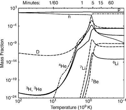
Fig. 4.16
The evolution of abundances of the light
elements formed in BBN, as a function of temperature (lower axis)
and cosmic time t (upper
axis). The decrease in neutron abundance in the first ∼ 3 min is
due to neutron decay. The density of deuterium increases
steeply—linked to the steep decrease in neutron density—and reaches
a maximum at t ∼ 3 min
because then its density becomes sufficiently large for efficient
formation of He4 to set in. Only a few deuterium nuclei
do not find a reaction partner and remain, with a mass fraction
of ∼ 10−5. Only a few other light nuclei are formed in
the Big Bang, mainly He3 and Li7. Source: D.
Tytler, J.M. O’Meara, N. Suzuki & D. Lubin 2000, Deuterium and the baryonic density of the
universe, Phys. Rep. 333, 409–432. Reprinted with permission
from Elsevier
Dependence of the
primordial abundances on the baryon density. At the end of
the first 3 min, the composition of the baryonic component of our
Universe is about as follows: 25 % of the baryonic mass is bound in
helium nuclei, 75 % in hydrogen nuclei (i.e., protons), with traces
of D, He3 and Li7. Heavier nuclei cannot form
because no stable nucleus of mass number 5 or 8 exists and thus no
new, stable nuclei can be formed in collisions of two helium nuclei
or of a proton with a helium nucleus. Collisions between three
nuclei are far too rare to contribute to nucleosynthesis. The
density in He4 and D depends on the baryon density in
the Universe, as can be seen in Fig. 4.17 and through the
following considerations:
-
A similar argument is valid for the abundance of deuterium: the larger Ω b is, the higher the baryon density during the conversion of D into He4. Thus the conversion will be more efficient and more complete. This means that fewer deuterium nuclei remain without a reaction partner for helium formation. Thus fewer of them are left over in the end, so the fraction of D will be lower.
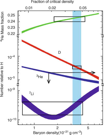
Fig. 4.17
BBN predictions of the primordial
abundances of light elements as a function of today’s baryon
density (ρ b, 0,
lower axis) and the corresponding density parameter Ω b where h = 0. 65 was assumed. The vertical
extent of the rectangles marks the measured values of the
abundances (top:
He4, center: D,
bottom: Li7).
The horizontal extent results from the overlap of these intervals
with curves computed from theoretical models. The ranges in
Ω b that are
allowed by these three species do overlap, as is indicated by the
vertical strip. The deuterium measurements yield the most stringent
constraints for Ω
b. Source: D. Tytler, J.M. O’Meara, N. Suzuki & D.
Lubin 2000, Deuterium and the
baryonic density of the universe, Phys. Rep. 333, 409–432.
Reprinted with permission from Elsevier
Baryon content of
the Universe. From measurements of the primordial abundances
of He4 and D and their comparison with detailed models
of nucleosynthesis in the early Universe, η or Ω b, respectively, can be
determined (see Fig. 4.17). The abundance of deuterium is a
particularly sensitive measure for Ω b. Measurements of the
relative strength of the Lyα lines of H and D, which have slightly
different transition frequencies due to the different masses of
their nuclei, in QSO absorption lines (see Sect. 5.7) yields  . Since the
intergalactic gas producing these absorption lines is very
metal-poor and thus presumably barely affected by nucleosynthesis
in stars, its D/H-ratio should be close to the primordial value.
Combining the quoted value of D/H with the model curves shown in
Fig. 4.17 we
find
. Since the
intergalactic gas producing these absorption lines is very
metal-poor and thus presumably barely affected by nucleosynthesis
in stars, its D/H-ratio should be close to the primordial value.
Combining the quoted value of D/H with the model curves shown in
Fig. 4.17 we
find
 With a Hubble constant of
  , thus
h 2 ≈ 1∕2, we
have Ω
b ≈ 0. 04. But since Ω m > 0. 1, this result
implies that baryons represent only a small fraction of the matter
in the Universe. The major
fraction of matter is non-baryonic dark matter.
, thus
h 2 ≈ 1∕2, we
have Ω
b ≈ 0. 04. But since Ω m > 0. 1, this result
implies that baryons represent only a small fraction of the matter
in the Universe. The major
fraction of matter is non-baryonic dark matter.
. Since the
intergalactic gas producing these absorption lines is very
metal-poor and thus presumably barely affected by nucleosynthesis
in stars, its D/H-ratio should be close to the primordial value.
Combining the quoted value of D/H with the model curves shown in
Fig. 4.17 we
find
(4.68)
, thus
h 2 ≈ 1∕2, we
have Ω
b ≈ 0. 04. But since Ω m > 0. 1, this result
implies that baryons represent only a small fraction of the matter
in the Universe. The major
fraction of matter is non-baryonic dark matter.To circumvent the conclusion of a dominant
fraction of non-baryonic matter, inhomogeneous models of BBN have
been investigated, but these also yield values for Ω b which are too low and
therefore do not provide a viable alternative.
Dependence of BBN
on the number of neutrino flavors. In the analysis of BBN we
implicitly assumed that not more than three (relativistic, i.e.,
with m ν < 1 MeV) neutrino families
exist. If N
ν > 3, the
quantitative predictions of BBN will change. In this case, the
expansion would occur faster [see (4.59)] because
ρ(T) would be larger, leaving less time
until the temperature has cooled down to T D—thus, fewer neutrons
would decay and the resulting helium abundance would be higher.
Even before 1990, it was concluded from BBN (with relatively large
uncertainties, however) that N ν = 3. In 1990, the value of
N ν = 3 was then confirmed in the
laboratory from Z-boson decay.
4.4.6 WIMPs as dark matter particles
There is a wide variety of evidence for the
existence of dark matter, from scales of individual galaxies
(rotation curves of spirals), clusters (velocity dispersion of
galaxies, X-ray temperature, lensing), to cosmological scales,
where the baryon density as inferred from BBN is lower than the
lower bound on the total matter density. The MACHO experiments
described in Sect. 2.5.3 rule out astronomical objects
as the dominant contribution to dark matter, at least in the halo
of the Milky Way; furthermore, all obvious candidates for
astronomical dark matter objects would yield very strong conflicts
with observations, for example concerning metallicity. In addition,
the fact that the mass density in the Universe is ∼ 6 times higher
than the baryonic density precludes any ‘normal’ astronomical
objects as the main constituent of dark matter. Therefore, the
solution of the dark matter issue must likely come from particle
physics.
Constraints on the
dark matter particle. Since dark matter particles are ‘dark’
they must be electrically neutral in order not to interact
electromagnetically. Furthermore, the particle must be stable, or
at least have a lifetime much longer than the age of the Universe,
so that they are still around today. The only known neutral
particles in the Standard Model (see Sect. 4.4.1) are the neutrinos
and the neutron. However, the neutron is baryonic, and its density
in the early Universe is very well constrained by BBN (see
Sect. 4.4.5);
furthermore, the free neutron is unstable and thus clearly not a
viable dark matter candidate. The neutrinos in principle could be
good dark matter candidates if they have a finite mass, since we
know they exist, and we actually know their abundance and their
temperature, which were determined at their decoupling—see
Sect. 4.4.3.
But they would be hot dark matter, and as such lead to a
large-scale structure in the Universe that would be very different
from the one we observe, as will be explained in more detail in
Sect. 7.4.1. In particular, they would be
too ‘hot’ to cluster on scales of galaxies, with their thermal
velocity exceeding that of the escape velocity from galaxy halos.
We thus conclude that none of the known particles is a viable dark
matter candidate.
Physics beyond the
Standard Model. This Standard Model of particle physics has
proved extremely successful in describing subatomic physics, as
discussed in Sect. 4.4.1. Predictions of low-energy
electromagnetic phenomena agree with laboratory measurements to
better than one part in a billion, and for electro-weak
interactions, the agreement is better than 10−3. Because
of its strengths and of non-linearities, strong interactions are
far more difficult to describe quantitatively from first
principles, and thus the strong interaction sector of the standard
model—quantum chromodynamics (QCD)—is less accurately tested than
the weak and electromagnetic part.
Despite its successes, the standard model is
known to be incomplete, and in at least one aspect, it directly
conflicts with observations: According to the standard model,
neutrinos should be massless. However, the Solar neutrino problem
and its solution has shown this to be not the case: The (electron)
neutrinos generated through nuclear fusion in the center of the Sun
can escape, due to their small interaction cross section. These
Solar neutrinos can be detected in (big!) terrestrial
detectors.10
However, the measured rate of electron neutrinos from the Sun is
only half as large as expected from Solar models. This Solar neutrino problem kept physicists
and astrophysicists busy for decades. Its solution consists of a
purely quantum-mechanical process, that of neutrino oscillations.
It it possible that during its propagation, an electron neutrino
transforms into a muon or tau neutrino, and back again. The
existence of such oscillations was speculated for a long time, and
provides a possible explanation for the missing rate of Solar
electron neutrinos. Indeed, in 2001 the Sudbury Neutrino
Observatory showed that neutrinos of all three flavors are received
from the Sun, and that the sum of the rates of these neutrinos is
compatible with the predicted rate from Solar models. In the
meantime, these neutrino oscillation have also been observed in
terrestrial experiments with neutrino beams.
Whereas neutrino oscillations are therefore well
established today, they are in conflict with the Standard Model,
according to which neutrinos have zero rest mass. From Special
Relativity one can easily show that massless particles can not
change their ‘identity’ while propagating through space. The
existence of neutrino oscillations necessarily requires that
neutrinos have a finite rest mass. Indeed, the oscillation
experiments were able to constrain these masses, since they
determine the length-scale over which the flavor of neutrinos
changes—more precisely, it depends on the difference of their
squared mass m
i 2.
One finds that  ,
and
,
and  .
These squared-mass differences thus do not provide us with an
absolute mass scale of neutrinos, but their mass is non-zero. That
means that neutrinos contribute to the cosmic matter density today,
giving a contribution of
.
These squared-mass differences thus do not provide us with an
absolute mass scale of neutrinos, but their mass is non-zero. That
means that neutrinos contribute to the cosmic matter density today,
giving a contribution of
 which depends only on the sum of the three neutrino masses—since
the number density of neutrinos is known from the thermal history
after the Big Bang. If the neutrino masses take the lowest values
allowed by the squared-mass differences given above, this
contribution is about 0.1 %. We will see in Chap. 8 that observations of the
large-scale structure in the Universe show that neutrinos cannot
contribute a substantial fraction to the matter density. Indeed,
these observations yield a constraint of
which depends only on the sum of the three neutrino masses—since
the number density of neutrinos is known from the thermal history
after the Big Bang. If the neutrino masses take the lowest values
allowed by the squared-mass differences given above, this
contribution is about 0.1 %. We will see in Chap. 8 that observations of the
large-scale structure in the Universe show that neutrinos cannot
contribute a substantial fraction to the matter density. Indeed,
these observations yield a constraint of  , and thus
the upper bound on neutrino masses from cosmology are much stricter
than those obtained from laboratory experiments. For the electron
neutrino, an upper limit on its mass was determined from decay
experiments of tritium, yielding
, and thus
the upper bound on neutrino masses from cosmology are much stricter
than those obtained from laboratory experiments. For the electron
neutrino, an upper limit on its mass was determined from decay
experiments of tritium, yielding  ,
which together with the results from neutrino oscillations implies
a maximum density of Ω
ν
< 0. 12.
,
which together with the results from neutrino oscillations implies
a maximum density of Ω
ν
< 0. 12.
,
and .
These squared-mass differences thus do not provide us with an
absolute mass scale of neutrinos, but their mass is non-zero. That
means that neutrinos contribute to the cosmic matter density today,
giving a contribution of
(4.69)
, and thus
the upper bound on neutrino masses from cosmology are much stricter
than those obtained from laboratory experiments. For the electron
neutrino, an upper limit on its mass was determined from decay
experiments of tritium, yielding ,
which together with the results from neutrino oscillations implies
a maximum density of Ω
ν
< 0. 12.Physical
motivation for WIMPs. Hence, the Standard Model needs an
extension which allows the existence of a finite neutrino mass. In
addition, there are other issues with the Standard Model—it is
“technically unnatural” since the energy scale of the Higgs
boson, ∼ 125 GeV, which is also comparable to the electro-weak mass
scale, i.e., the masses of the W and Z bosons, is so much smaller
than the Planck mass,11 and it can also not explain why
there are more baryons than anti-baryons in the current Universe.
The former of these problems is called the gauge hierarchy problem;
in order to solve it, one needs some new physics at an energy scale
of ∼ 100 GeV. There are several models, extending the Standard
Model, which introduce new physics at this scale. Arguably, the
most promising of those is supersymmetry.
Then suppose that in the extended model, there
exists a electrically neutral particle X which is stable, has a
mass of order the energy scale of the model, i.e., somewhere
between 100 GeV and 10 TeV, and interacts only weakly.12 Such Weakly Interacting
Massive Particles (WIMPs) are the most promising dark matter
candidates—because, if such a particle exists, it would have the
right cosmic density to account for the dark matter.
At first sight, it may be difficult to see how
one can estimate the cosmic mass density of a particle whose
existence and properties are as yet unknown, but indeed we can. For
that, recall how we obtained the abundance of neutrinos in the
Universe. Above a certain temperature, they were in thermodynamic
equilibrium with the rest of the matter in the Universe, but when
their interaction rate became too slow, they dropped out of
equilibrium with the rest of the matter in the Universe, and kept
their comoving number density from then on.
Now, let’s assume the WIMP particle X exists. At
sufficiently early times, it was in thermodynamic equilibrium.
Since it is weakly interacting by assumption, we have a good idea
about its cross section, and thus conclude that it stays in
equilibrium during the phase when the temperature of the Universe
drops below  ,
i.e., when the particles become non-relativistic. Once this
happens, the equilibrium number density is determined by the
Boltzmann factor,
,
i.e., when the particles become non-relativistic. Once this
happens, the equilibrium number density is determined by the
Boltzmann factor,
 and thus starts to decrease rapidly with decreasing T. At T ≈ 0. 05m X, the interaction rate of
X becomes too small to keep them in equilibrium with the other
particles present, they freeze out, and from then on have constant
comoving number density. Their mass density is then easily obtained
as the product of their number density and m X. Amazingly, if
m X ≈ 300 GeV,
the resulting density of these WIMPs would yield
and thus starts to decrease rapidly with decreasing T. At T ≈ 0. 05m X, the interaction rate of
X becomes too small to keep them in equilibrium with the other
particles present, they freeze out, and from then on have constant
comoving number density. Their mass density is then easily obtained
as the product of their number density and m X. Amazingly, if
m X ≈ 300 GeV,
the resulting density of these WIMPs would yield  ,
with an uncertainty of about a factor ∼ 3 (owing to the as yet
unknown detailed properties and thus the precise value of the
interaction cross section of X).
,
with an uncertainty of about a factor ∼ 3 (owing to the as yet
unknown detailed properties and thus the precise value of the
interaction cross section of X).
,
i.e., when the particles become non-relativistic. Once this
happens, the equilibrium number density is determined by the
Boltzmann factor,
,
with an uncertainty of about a factor ∼ 3 (owing to the as yet
unknown detailed properties and thus the precise value of the
interaction cross section of X).Hence, if a massive WIMP exists with properties
expected from particle theory—weakly interacting, and with a mass
near the weak interaction mass scale—the cosmological density of
these particles is just the observed dark matter density! This
indeed is an astonishing result, sometimes called the ‘WIMP
miracle’, a miracle perhaps too good to be just a random
coincidence. For that reason, such a WIMP is the favorite candidate
for the dark matter particle. Fortunately, this model can be
experimentally verified, and there are three ways how this can be
achieved.
Direct
detection. The first one is the direct detection. These
WIMPs, if they constitute the dark matter in our Galaxy, should
also be present in our neighborhood and pass through the Earth.
Since they are weakly interacting only, their cross section with
ordinary matter is very small, and they are difficult to detect.
Nevertheless, experiments were built to search for such particles
through their scattering with detector material, i.e., atomic
nuclei. Due to scattering, the WIMP will transfer a momentum to the
nucleus, and the resulting energy gain can be used for detection.
One can estimate the associated recoil energy, given a plausible
mass of ∼ 300 GeV and the characteristic velocity of ∼ 200 km∕s,
corresponding to typical velocities in the Galaxy. Then, the
kinematics of the scattering process implies that the recoil energy
is small, ∼ 100 keV. This energy causes a tiny temperature increase
of the detector, which must be probed.
Several different methods for the WIMP detection
have been turned into experiments. Since WIMP events will be rare,
one needs to place the detectors in a well-shielded environment, in
laboratories deep underground, so that the background of cosmic ray
particles is strongly suppressed. In order to test whether a
measured signal is indeed due to particles from outside the Solar
system, one checks for an annual variation: Due to the orbit of the
Earth around the Sun, our velocity relative to the Galactic frame
changes over the year, and the event rate should behave
accordingly.
Existing experiments have imposed bounds on
combinations of the WIMP mass and its cross section, and ruled out
a significant fraction of plausible parameter space. Improvements
in the experiments give rise to the expectation that WIMPs can be
detected within the next few years. In fact, some experiments have
claimed a detection, and also saw an annual modulation. However,
the corresponding estimates of the mass and cross section are ruled
out by other experiments, so that the interpretation of these
results is controversial at present.
Particle
colliders. The Large Hadron Collider (LHC) at CERN started
operation in 2009; its two major science drivers were the search
for the Higgs particle, which has been achieved in the meantime,
and the search for phenomena beyond the Standard Model of particle
physics. As we argued before, there are good reasons to assume that
new physics will appear beyond ∼ 100 GeV, an energy range probed by
the LHC. However, although the LHC will probably be able to produce
WIMPs—if they exist—it will not lead to a direct WIMP detection,
due to the low interaction cross sections with matter. Therefore,
indirect methods must be used. For example, if supersymmetry is the
correct extension of the Standard Model, supersymmetric particles
will be produced and decay in the detector, thereby producing the
lightest supersymmetric particle—presumably the WIMP. From adding
up the charges, momenta and energy of all particles in the
reaction, one could then conclude that a neutral particle has left
the detector, and get an estimate on its mass. This particle must
have a lifetime of ∼ 10−7 s in order not to decay inside
the detector. This lower bound on the lifetime is far away from the
requested lifetime  of the WIMP. Therefore,
even though the LHC may point towards the correct physical nature
of the WIMP candidate, only its direct detection can prove that it
is indeed the dark matter particle. However, from the measured
cross sections of other supersymmetric particles, one can determine
the free parameters of the model (at least in its simplest
version), and from that get an estimate of the WIMP annihilation
cross section. Since this, in combination with the WIMP mass,
determines its cosmological density, as explained above,
Ω X can be
estimated in the laboratory! If this value agrees with
of the WIMP. Therefore,
even though the LHC may point towards the correct physical nature
of the WIMP candidate, only its direct detection can prove that it
is indeed the dark matter particle. However, from the measured
cross sections of other supersymmetric particles, one can determine
the free parameters of the model (at least in its simplest
version), and from that get an estimate of the WIMP annihilation
cross section. Since this, in combination with the WIMP mass,
determines its cosmological density, as explained above,
Ω X can be
estimated in the laboratory! If this value agrees with  ,
then this neutral particle will be indeed an excellent candidate
for the dark matter.
,
then this neutral particle will be indeed an excellent candidate
for the dark matter.
of the WIMP. Therefore,
even though the LHC may point towards the correct physical nature
of the WIMP candidate, only its direct detection can prove that it
is indeed the dark matter particle. However, from the measured
cross sections of other supersymmetric particles, one can determine
the free parameters of the model (at least in its simplest
version), and from that get an estimate of the WIMP annihilation
cross section. Since this, in combination with the WIMP mass,
determines its cosmological density, as explained above,
Ω X can be
estimated in the laboratory! If this value agrees with ,
then this neutral particle will be indeed an excellent candidate
for the dark matter.Indirect
astrophysical detections. In its simplest form, we expect
from supersymmetry that the WIMP is its own anti-particle, and thus
two WIMPs can annihilate. That happened in the early Universe
before the freeze-out of WIMPs, but since then became very rare.
Nevertheless, in regions of high dark matter density, some
annihilation may occur. The resulting signal depends on the kind of
particles into which they annihilate, but in general one would
expect that high-energy photons are generated in the decay chain,
which may be visible in hard γ-radiation. The number density of
annihilation events is proportional to the square of the WIMP
density, and therefore the most promising places to look for these
γ-rays are probably the
centers of dark matter halos—in particular, the center of the
Galaxy and that of nearby dwarf galaxies. Of course, the problem of
distinguishing the annihilation signal from other γ-ray sources needs to be
overcome.
Another indirect method is based on the fact that
some WIMPs which cross the Earth or the Sun get scattered by atomic
nuclei, thereby change their velocity, which may become lower than
the escape velocity from these objects, and thus they are
gravitationally captured. After that, they will orbit within the
Sun (or the Earth), and due to the high density there, they will
scatter again, and finally sink toward the center of the body.
Therefore, the density of WIMPs can be strongly enhanced there, and
correspondingly the rate of annihilations. The annihilation
products will decay, or be stopped, in the body, except for
neutrinos which escape. The signature of the annihilation are thus
neutrinos, with an energy much higher that produced in nuclear
fusion processes. Hence, such high-energy neutrino signals from the
center of the Earth or the Sun would be a unique signature of WIMP
annihilation. Existing neutrino detectors, such as IceCube in
Antarctica, are beginning to probe interesting regions in the WIMP
parameter space of mass and cross section.
4.4.7 Recombination
About 3 min after the Big Bang, BBN comes to an
end. At this time, the Universe has a temperature of roughly
T ∼ 8 × 10⁸ K
and consists of photons, protons, helium nuclei, traces of other
light elements, and electrons. In addition, there are neutrinos
that dominate, together with photons, the energy density and thus
also the expansion rate, and there are (probably) WIMPs. Except for
the neutrinos and the WIMPs, all particle species have the same
temperature, which is established by interactions of charged
particles with the photons, which resemble some kind of heat
bath.
At  ,
pressureless matter (i.e., the so-called dust) begins to dominate
the cosmic energy density and thus the expansion rate. The second
term in (4.33) then becomes largest, i.e.,
,
pressureless matter (i.e., the so-called dust) begins to dominate
the cosmic energy density and thus the expansion rate. The second
term in (4.33) then becomes largest, i.e.,  .
If a power-law ansatz for the scale factor, a ∝ t β , is inserted into the
expansion equation, we find that
.
If a power-law ansatz for the scale factor, a ∝ t β , is inserted into the
expansion equation, we find that  , and hence
 This describes the expansion behavior until either the curvature
term or, if this is zero or very small, the Λ-term starts to dominate.
This describes the expansion behavior until either the curvature
term or, if this is zero or very small, the Λ-term starts to dominate.
,
pressureless matter (i.e., the so-called dust) begins to dominate
the cosmic energy density and thus the expansion rate. The second
term in (4.33) then becomes largest, i.e., .
If a power-law ansatz for the scale factor, a ∝ t β , is inserted into the
expansion equation, we find that , and hence
(4.70)
After further cooling, the free electrons can
combine with the nuclei and form neutral atoms. This process is
called recombination,
although this expression is misleading: since the Universe was
fully ionized until then, it is not a recombination but rather the (first)
transition to a neutral state—however the expression
‘recombination’ has now long been established. The recombination of
electrons and nuclei is in competition with the ionization of
neutral atoms by energetic photons (photoionization), whereas
collisional ionization can be disregarded completely since
η—see (4.65)—is so small.
Because photons are so much more numerous than electrons, cooling
has to proceed to well below the ionization temperature,
corresponding to the binding energy of an electron in hydrogen,
before neutral atoms become abundant. This happens for the same
reasons as apply in the context of deuterium formation: there are
plenty of ionizing photons in the Wien tail of the Planck
distribution, even if the temperature is well below the ionization
temperature. The ionization energy of hydrogen is χ = 13. 6 eV, corresponding to a
temperature of T > 105 K, but
T has to first decrease
to ∼ 3000 K before the ionization fraction
 falls considerably below 1, for the reason mentioned above. At
temperatures T > 104 K we have
x ≈ 1, i.e., virtually all
electrons are free. Only below z ∼ 1300 does x deviate significantly from
unity.
falls considerably below 1, for the reason mentioned above. At
temperatures T > 104 K we have
x ≈ 1, i.e., virtually all
electrons are free. Only below z ∼ 1300 does x deviate significantly from
unity.
(4.71)
The onset of recombination can be described by an
equilibrium consideration which leads to the so-called Saha
equation ,
 which describes the ionization fraction x as a function of temperature.
However, once recombination occurs, the assumption of
thermodynamical equilibrium is no longer justified. This can be
seen as follows:
which describes the ionization fraction x as a function of temperature.
However, once recombination occurs, the assumption of
thermodynamical equilibrium is no longer justified. This can be
seen as follows:
Any recombination directly to the ground state
leads to the emission of a photon with energy E γ > χ. However, these photons can ionize
other, already recombined (thus neutral), atoms. Because of the
large cross section for photoionization, this happens very
efficiently. Thus for each recombination to the ground state, one
neutral atom will become ionized, yielding a vanishing net effect.
But recombination can also happen in steps, first into an excited
state and then evolving into the ground state by radiative
transitions. Each of these recombinations will yield a Lyman-series
photon in the transition from an excited state into the ground
state. This Lyman photon will then immediately excite another atom
from the ground state into an excited state, which has an
ionization energy of ≤ χ∕4.
This yields no net production of atoms in the ground state. Since
the density of photons with E γ > χ∕4 is very much larger than of those
of E γ > χ, the excited atoms are more easily
ionized, and this indeed happens. Stepwise recombination thus also
provides no route towards a lower ionization fraction.
The processes described above cause a small
distortion of the Planck spectrum due to recombination radiation
(in the range χ ≫ k B T) which affects recombination. One
cannot get rid of these energetic photons—in contrast to gas
nebulae like Hii
regions, in which the Lyα
photons may escape due to the finite geometry.
Fig. 4.18
The first lines of the article by Penzias
and Wilson (1965), ApJ 142, 419
Ultimately, recombination takes place by means of
a very rare process, the two-photon decay of the first excited
level. This process is less probable than the direct Lyα transition by a factor
of ∼ 108. However, it leads to the emission of two
photons, neither of which is sufficiently energetic to excite an
atom from the ground state. This 2γ-transition is therefore a net sink
for energetic photons.13 Taking into account all relevant
processes and using a rate equation, which describes the evolution
of the distribution of particles and photons even in the absence of
thermodynamic equilibrium, gives for the ionization fraction in the
relevant redshift range 
 The ionization fraction is thus a very strong function of redshift
since x changes from 1
(complete ionization) to x ∼ 10−4 (where essentially
all atoms are neutral) within a relatively small redshift range.
The recombination process is not complete, however. A small
ionization fraction of x ∼ 10−4 remains since the
recombination rate for small x becomes smaller than the expansion
rate—some nuclei do not find an electron fast enough before the
density of the Universe becomes too low. From (4.72), the optical depth
for Thomson scattering (scattering of photons by free electrons)
can be computed (see problem 4.12),
The ionization fraction is thus a very strong function of redshift
since x changes from 1
(complete ionization) to x ∼ 10−4 (where essentially
all atoms are neutral) within a relatively small redshift range.
The recombination process is not complete, however. A small
ionization fraction of x ∼ 10−4 remains since the
recombination rate for small x becomes smaller than the expansion
rate—some nuclei do not find an electron fast enough before the
density of the Universe becomes too low. From (4.72), the optical depth
for Thomson scattering (scattering of photons by free electrons)
can be computed (see problem 4.12),
 which is virtually independent of cosmological parameters.
Equation (4.73) implies that photons can propagate from
z ∼ 1000 (the ‘last-scattering surface’) until the
present day essentially without any interaction with
matter—provided the wavelength is larger than 1216 Å. For photons
of smaller wavelength, the absorption cross section of neutral
atoms is large. Disregarding these highly energetic photons
here—their energies are
which is virtually independent of cosmological parameters.
Equation (4.73) implies that photons can propagate from
z ∼ 1000 (the ‘last-scattering surface’) until the
present day essentially without any interaction with
matter—provided the wavelength is larger than 1216 Å. For photons
of smaller wavelength, the absorption cross section of neutral
atoms is large. Disregarding these highly energetic photons
here—their energies are  , compared to T rec ∼ 0. 3 eV, so they are
far out in the Wien tail of the Planck distribution—we conclude
that the photons present after recombination have been able to
propagate without further interactions until the present epoch.
Before recombination they followed a Planck spectrum. As was
discussed in Sect. 4.3.2, the distribution will remain a Planck
spectrum with only its temperature changing. Thus these photons
from the early Universe should still be observable today,
redshifted into the microwave regime of the electromagnetic
spectrum.
, compared to T rec ∼ 0. 3 eV, so they are
far out in the Wien tail of the Planck distribution—we conclude
that the photons present after recombination have been able to
propagate without further interactions until the present epoch.
Before recombination they followed a Planck spectrum. As was
discussed in Sect. 4.3.2, the distribution will remain a Planck
spectrum with only its temperature changing. Thus these photons
from the early Universe should still be observable today,
redshifted into the microwave regime of the electromagnetic
spectrum.
(4.72)
(4.73)
, compared to T rec ∼ 0. 3 eV, so they are
far out in the Wien tail of the Planck distribution—we conclude
that the photons present after recombination have been able to
propagate without further interactions until the present epoch.
Before recombination they followed a Planck spectrum. As was
discussed in Sect. 4.3.2, the distribution will remain a Planck
spectrum with only its temperature changing. Thus these photons
from the early Universe should still be observable today,
redshifted into the microwave regime of the electromagnetic
spectrum.Our consideration of the early
Universe predicts thermal radiation from the Big Bang, as was first
realized by George Gamow in 1946—the cosmic microwave background.
The CMB is therefore a visible relic of the Big Bang.
The CMB was detected in 1965 by Arno Penzias
& Robert Wilson (see Fig. 4.18), who were awarded the 1978 Nobel prize in
physics for this very important discovery. At the beginning of the
1990s, the COBE satellite measured the spectrum of the CMB with a
very high precision—it is the most perfect blackbody ever measured
(see Fig. 4.3). From upper bounds of deviations from the
Planck spectrum, very tight limits for possible later energy
injections into the photon gas, and thus on energetic processes in
the Universe, can be obtained. 14
We have only discussed the recombination of
hydrogen. Since helium has a higher ionization energy it recombines
earlier than hydrogen. Although recombination defines a rather
sharp transition, (4.73) tells us that we receive photons from a
recombination layer of finite thickness (Δ z ∼ 60). This aspect will be of
importance later.
The gas in the intergalactic medium at lower
redshift is highly ionized. If this were not the case we would not
be able to observe any UV photons from sources at high redshift
(‘Gunn-Peterson-test’, see Sect. 8.5.1). Sources with redshifts
z > 6 have been
observed, and we also observe photons with wavelengths shorter than
the Lyα line of these
objects. Thus at least at the epoch corresponding to redshift
z ∼ 6, the Universe must
have been nearly fully ionized or else these photons would have
been absorbed by photoionization of neutral hydrogen. This means
that at some time between z ∼ 1000 and z ∼ 6, a reionization of the
intergalactic medium must have occurred, presumably by a first
generation of stars or by the first AGNs. The results from the new
CMB satellites WMAP and Planck suggest a reionization at redshift
z ∼ 10; this will be
discussed more thoroughly in Sect. 8.7.
4.4.8 Summary
We will summarize this somewhat long section as
follows:
-
Our Universe originated from a very dense, very hot state, the so-called Big Bang. Shortly afterwards, it consisted of a mix of various elementary particles, all interacting with each other.
-
We are able to examine the history of the Universe in detail, starting at an early epoch where it cooled down by expansion such as to leave only those particle species known to us (electrons, protons, neutrons, neutrinos, and photons), and probably a dark matter particle.
-
Because of their weak interaction and the decreasing density, the neutrinos experience only little interaction at temperatures below ∼ 1010 K, their decoupling temperature.
-
At T ∼ 5 × 10⁹ K, electrons and positrons annihilate into photons. At this low temperature, pair production ceases to take place.
-
Protons and neutrons interact and form deuterium nuclei. As soon as T ∼ 109 K, deuterium is no longer efficiently destroyed by energetic photons. Further nuclear reactions produce mainly helium nuclei. About 25 % of the mass in nucleons is transformed into helium, and traces of lithium are produced, but no heavier elements.
-
At about T ∼ 3000 K, some 400 000 years after the Big Bang, the protons and helium nuclei combine with the electrons, and the Universe becomes essentially neutral (we say that it ‘recombines’). From then on, photons can travel without further interactions. At recombination, the photons follow a blackbody distribution (i.e., a thermal spectrum, or a Planck distribution). By the ongoing cosmic expansion, the temperature of the spectral distribution decreases, T ∝ (1 + z), though its Planck property remains.
-
After recombination, the matter in the Universe is almost completely neutral. However, we know from the observation of sources at very high redshift that the intergalactic medium is essentially fully ionized at
 . Before z > 6, our Universe must therefore
have experienced a phase of reionization. This effect cannot be
explained in the context of the strictly homogeneous world models;
rather it must be examined in the context of structure formation in
the Universe and the formation of the first stars and AGNs. These
aspects will be discussed in Sect. 10.3.
. Before z > 6, our Universe must therefore
have experienced a phase of reionization. This effect cannot be
explained in the context of the strictly homogeneous world models;
rather it must be examined in the context of structure formation in
the Universe and the formation of the first stars and AGNs. These
aspects will be discussed in Sect. 10.3.
4.5 Achievements and problems of the standard model
To conclude this chapter, we will evaluate the
cosmological model which has been presented. We will review its
achievements and successes, but also apparent problems, and point
out the route by which those might be understood. As is always the
case in natural sciences, problems with an otherwise very
successful model are often the key to a new and deeper
understanding.
4.5.1 Achievements
The standard model of the Friedmann–Lemaître
universe described above has been extremely successful in numerous
ways:
-
It predicts that gas which has not been subject to much chemical processing (i.e., metal-poor gas) should have a helium content of ∼ 25 %. This is in extraordinarily good agreement with observations.
-
It predicts that sources of lower redshift are closer to us than sources of higher redshift.15 Therefore, modulo any peculiar velocities, the absorption of radiation from sources at high redshift must happen at smaller redshifts. Not a single counter-example has been found yet.
-
It predicts the existence of a microwave background, which indeed was found.
-
It predicts the correct number of neutrino families, which was confirmed in laboratory experiments of the Z-boson decay.
Further achievements will be discussed in the
context of structure evolution in the Universe.
A good physical model is one that can also be
falsified. In this respect, the Friedmann–Lemaître universe is also
an excellent model: a single observation could either cause a lot
of trouble for this model or even disprove it. To wit, it would be
incompatible with the model
1.
if the helium content of a gas cloud or of a
low-metallicity star was significantly below 25 %;
2.
if it was found that one of the neutrinos has a
rest mass  ;
;
;3.
if the Wien-part of the CMB had a smaller
amplitude compared to the Planck spectrum;
4.
if a source with emission lines at z e was found to show
absorption lines at  ;
;
;5.
if the cosmological parameters were such that
 .
.
.On (1): While the helium content may increase by
stellar evolution due to fusion of hydrogen into helium, only a
small fraction of helium is burned in stars. In this process,
heavier elements are of course produced. A gas cloud or a star with
low metallicity therefore cannot consist of material in which
helium has been destroyed; it must contain at least the helium
abundance from BBN. On (2): Such a neutrino would lead to
Ω m > 2,
which is in strict contradiction to the derived model parameters.
On (3): Though it is possible to generate additional photons by
energetic processes in the past, thereby increasing the Wien-part
of the coadded spectrum compared to that of a Planck function, it
is thermodynamically impossible to extract photons from the
Wien-part. On (4): Such an observation would question the role of
redshift as a monotonic measure of relative distances and thus
remove one of the pillars of the model. On (5): Our knowledge of
stellar evolution allows us to determine the age of the oldest
stars with a precision of better than ∼ 20 %. An age of the Universe
below ∼ 10 Gyr would be incompatible with the age of the globular
clusters—naturally, these have to be younger than the age of our
Universe, i.e., the time after the Big Bang.
Although these predictions have been known for
more than 40 years, no observation has yet been made which
disproves the standard model. Indeed, at any given time there have
been astronomers who like to disagree with the standard model.
These astronomers have tried to make a discovery, like the examples
above, which would pose great difficulties for the model. So far
without success; this does not mean that such results cannot be
found in the literature, but rather such results did not withstand
closer examination. The simple opportunities to falsify the model
and the lack of any corresponding observation, together with the
achievements listed above, have made the Friedmann–Lemaître model
the standard model of
cosmology. Alternative models have either been excluded by
observation (such as steady-state cosmology) or have been unable to
make any predictions. Currently, there is no serious alternative to
the standard model.
4.5.2 Problems of the standard model
Despite these achievements, there are some
aspects of the model which require further consideration. Here we
will describe two conceptual problems with the standard model more
thoroughly—the horizon problem and the flatness problem.
Horizons.
The finite speed of light implies that we are only able to observe
a finite part of the Universe, namely those regions from which
light can reach us within a time t 0. Since t 0 ≈ 13. 8 Gyr, our visible
Universe has—roughly speaking—a radius of 13.8 billion light years.
More distant parts of the Universe are at the present time
unobservable for us. This means that there exists a horizon beyond
which we cannot see. Such horizons do not only exist for us today:
at an earlier time t, the
size of the horizon was about ct, hence smaller than today. We will
now describe this aspect quantitatively.
In a time interval dt, light travels a distance
c dt, which corresponds to a comoving
distance interval  at scale factor
a. From the Big Bang to a
time t (or redshift
z) the light traverses a
comoving distance of
at scale factor
a. From the Big Bang to a
time t (or redshift
z) the light traverses a
comoving distance of
 From
From  we get
 ,
so that
,
so that
 If z
eq ≫ z ≫ 0, the
main contribution to the integral comes from times (or values of
a) in which pressureless
matter dominates the expansion rate H. Then with (4.33) we find
If z
eq ≫ z ≫ 0, the
main contribution to the integral comes from times (or values of
a) in which pressureless
matter dominates the expansion rate H. Then with (4.33) we find
 ,
and (4.74) yields
,
and (4.74) yields
 In earlier phases, z ≫ z eq, H is radiation-dominated,
  ,
and (4.74) becomes
,
and (4.74) becomes
 The earlier the cosmic epoch, the smaller the comoving horizon
length, as was to be expected. In particular, we will now consider
the recombination epoch, z
rec ∼ 1000, for which (4.75) applies (see
Fig. 4.19).
The comoving length r
H,com corresponds to a physical proper length
r
H,prop = a r H,com, and thus
The earlier the cosmic epoch, the smaller the comoving horizon
length, as was to be expected. In particular, we will now consider
the recombination epoch, z
rec ∼ 1000, for which (4.75) applies (see
Fig. 4.19).
The comoving length r
H,com corresponds to a physical proper length
r
H,prop = a r H,com, and thus
at scale factor
a. From the Big Bang to a
time t (or redshift
z) the light traverses a
comoving distance of
we get
,
so that
(4.74)
,
and (4.74) yields
(4.75)
,
and (4.74) becomes
(4.76)
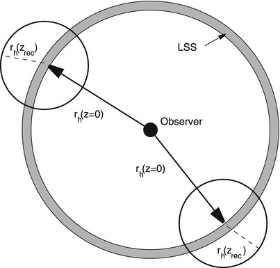
Fig. 4.19
The horizon problem: the region of space
which was in causal contact before recombination has a much smaller
radius than the spatial separation between two regions from which
we receive the CMB photons. Thus the question arises how these two
regions may ‘know’ of each other’s temperature. Adapted from: Alan
Guth 1998, The inflationary Universe, Basic Books

(4.77)


(4.78)
The horizon problem: Since no signal can
travel faster than light, (4.78) means that CMB radiation from two
directions separated by more than about one degree originates in
regions that were not in causal contact before recombination, i.e.,
the time when the CMB photons interacted with matter the last time.
Therefore, these two regions have never been able to exchange
information, for example about their temperature. Nevertheless
their temperature is the same, as seen from the high degree of
isotropy of the CMB, which shows relative fluctuations of only
 !
!
!Redshift-dependent
density parameter. We have defined the density parameters
Ω m and
Ω Λ as the current density divided
by the critical mass density ρ cr today. These
definitions can be generalized. If we existed at a different time,
the densities and the Hubble constant would have had different
values and consequently we would obtain different values for the
density parameters. Thus we define the total density parameter for
an arbitrary redshift
 where the critical density ρ cr is also a function of
redshift,
where the critical density ρ cr is also a function of
redshift,
 Then by inserting (4.24) into (4.79), we find
 Using (4.33), this yields
![$$\displaystyle{ \fbox{$1 -\varOmega _{0}(z) = F\,\left [1 -\varOmega _{0}(0)\right ]$}\;, }$$](A129044_2_En_4_Chapter_Equ82.gif) where Ω 0(0) is
the total density parameter today, and
where Ω 0(0) is
the total density parameter today, and
 From (4.81) we can now draw two important
conclusions. Since F > 0
for all a, the sign of
(Ω 0 − 1) is
preserved and thus is the same at all times as today. Since the
sign of (Ω 0 −
1) is the same as that of the curvature—see (4.32)—the sign of the
curvature is preserved in cosmic evolution: a flat Universe will be
flat at all times, a closed Universe with K > 0 will always have a positive
curvature.
From (4.81) we can now draw two important
conclusions. Since F > 0
for all a, the sign of
(Ω 0 − 1) is
preserved and thus is the same at all times as today. Since the
sign of (Ω 0 −
1) is the same as that of the curvature—see (4.32)—the sign of the
curvature is preserved in cosmic evolution: a flat Universe will be
flat at all times, a closed Universe with K > 0 will always have a positive
curvature.
(4.79)
(4.80)
(4.81)
(4.82)
The second conclusion follows from the analysis
of the function F at early
cosmic epochs, e.g., at z ≫ z eq, thus in the
radiation-dominated Universe. Back then, with (4.33), we have
 so that for very early times, F becomes very small. For instance, at
z ∼ 1010, the
epoch of neutrino freeze-out,
so that for very early times, F becomes very small. For instance, at
z ∼ 1010, the
epoch of neutrino freeze-out,  . Today, Ω 0 is of order unity; from
observations, we know that certainly
. Today, Ω 0 is of order unity; from
observations, we know that certainly  , where
this is a very generous
estimate,16 so that
, where
this is a very generous
estimate,16 so that
 .
Since F is so small at
large redshifts, this means that Ω 0(z) must have been very, very close to
1; for example at z ∼ 1010 it is required that
.
Since F is so small at
large redshifts, this means that Ω 0(z) must have been very, very close to
1; for example at z ∼ 1010 it is required that
 .
.
. Today, Ω 0 is of order unity; from
observations, we know that certainly , where
this is a very generous
estimate,16 so that
.
Since F is so small at
large redshifts, this means that Ω 0(z) must have been very, very close to
1; for example at z ∼ 1010 it is required that
.Flatness problem: For the total density
parameter to be of order unity today, it must have been extremely
close to 1 at earlier times, which means that a very precise ‘fine
tuning’ of this parameter was necessary.
This aspect can be illustrated very well by
another physical example. If we throw an object up into the air, it
takes several seconds until it falls back to the ground. The higher
the initial velocity, the longer it takes to hit the ground. To
increase the time of flight we need to increase the initial
velocity, for instance by using a cannon. In this way, the time of
flight may be extended to up to about a minute. Assume that we want
the object to be back only after one day; in this case we must use
a rocket. But we know that if the initial velocity of a rocket
exceeds the escape velocity v esc ∼ 11. 2 km∕s, it will
leave the gravitational field of the Earth and never fall back. On
the other hand, if the initial velocity is too much below
v esc, the
object will be back in significantly less than a day. So the
initial velocity must be very well chosen for the object to
return after being up for at least a day. The flatness problem is
completely analogous to this.
Let us consider the consequences of the case
where Ω 0 had
not been so extremely close to 1 at z ∼ 1010; then, the universe
would have recollapsed long ago, or it would have expanded
significantly faster than the universe we live in. In either case,
the consequences for the evolution of life in the universe would
have been catastrophic. In the first case, the total lifetime of
the universe would have been much shorter than is needed for the
formation of the first stars and the first planetary systems, so
that in such a world no life could be formed. In the second case,
extreme expansion would have prevented the formation of structure
in the universe. In such a universe no life could have evolved
either.
This consideration can be interpreted as follows:
we live in a universe which had, at a very early time, a very
precisely tuned density parameter, because only in such a universe
can life evolve and astronomers exist to examine the flatness of
the universe. In all other conceivable universes this would not be
possible. This approach is meaningful only if a large number of
universes existed—in this case we should not be too surprised about
living in one of those where this initial fine-tuning took place—in
the other ones, we, and the question about the cosmological
parameters, would just not exist. This approach is called the
anthropic principle. It may
either be seen as an ‘explanation’ for the flatness of our Universe, or as a
capitulation—where we give up to explore a physical reason for the
origin of the flatness of our Universe.
The example of the rocket given above is helpful
in understanding another aspect of cosmic expansion. If the rocket
is supposed to have a long time of flight but not escape the
gravitational field of the Earth, its initial velocity must be
very, very close to, but a tiny little bit smaller than
v esc. In other
words, the absolute value of the sum of kinetic and potential
energy has to be very much smaller than either of these two
components. This is also true for a large part of the initial
trajectory. Independent of the exact value of the time of flight,
the initial trajectory can be approximated by the limiting case
v
0 = v
esc at which the total energy is exactly zero.
Transferred to the Hubble expansion, this reads as follows:
independent of the exact values of the cosmological parameters, the
curvature term can be disregarded in the early phases of expansion
(as we have already seen above). This is because our Universe can
reach its current age only if at early times the modulus of
potential and kinetic energy were nearly exactly equal, i.e., the
curvature term in (4.14) must have been a lot smaller than the
other two terms.
4.5.3 Extension of the standard model: inflation
We will consider the horizon and flatness
problems from a different, more technical point of view. Einstein’s
field equations of GR, one solution of which has been described as
our world model, are a system of coupled partial differential
equations. As is always the case for differential equations, their
solutions are determined by (1) the system of equations itself and
(2) the initial conditions. If the initial conditions at, e.g.,
t = 1 s were as they have
been described, the two aforementioned problems would not exist.
But why are the conditions at t = 1 s such that they lead to a
homogeneous, isotropic, (nearly) flat model? The set of homogeneous
and isotropic solutions to the Einstein equation is of measure zero
(i.e., nearly all solutions of the Einstein equation are not
homogeneous and isotropic); thus these particular solutions are
very special. Taking the
line of reasoning that the initial conditions ‘just happened to be
so’ is not satisfying because it does not explain anything. Besides
the anthropic principle, the answer to this question can only be
that processes must have taken place even earlier, due to known or
as yet unknown physics, which have produced these ‘initial
conditions’ at t = 1 s. The
initial conditions of the normal Friedmann–Lemaître expansion thus
have a physical origin. Cosmologists believe they have found such a
physical reason: the inflationary model.
Inflation.
In the early 1980s, a model was developed which was able to solve
the flatness and horizon problems (and some others as well). As a
motivation for this model, we first recall that the physical laws
and properties of elementary particles are well known up to
energies of ∼ 100 GeV because they were experimentally tested in
particle accelerators. For higher energies, particles and their
interactions are unknown. This means that the history of the
Universe, as sketched above, can be considered secure only up to
energies of 100 GeV. The extrapolation to earlier times, up to the
Big Bang, is considerably less certain. From particle physics we
expect new phenomena to occur at an energy scale of the Grand
Unified Theories (GUTs), at about 1014 GeV,
corresponding to t ∼ 10−34 s.
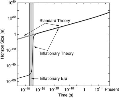
Fig. 4.20
During an inflationary phase, indicated
here by the gray bar, the
universe expands exponentially; see (4.83). This phase comes
to an end when a phase transition transforms the vacuum energy into
matter and radiation, after which the universe follows the normal
Friedmann expansion. Adapted from: Alan Guth 1998, The inflationary
Universe, Basic Books
In the inflationary scenario it is presumed that
at very early times the vacuum energy density was much higher than
today, so that it dominated the Hubble expansion. Then
from (4.18) we find that  . This
implies an exponential expansion of the Universe,
. This
implies an exponential expansion of the Universe,
 Obviously, this exponential expansion (or inflationary phase)
cannot last forever. We assume that a phase transition took place
in which the vacuum energy density is transformed into normal
matter and radiation (a process called reheating), which ends the
exponential expansion and after which the normal Friedmann
evolution of the Universe begins. Figure 4.20 sketches the
expansion history of the universe in an inflationary model.
Obviously, this exponential expansion (or inflationary phase)
cannot last forever. We assume that a phase transition took place
in which the vacuum energy density is transformed into normal
matter and radiation (a process called reheating), which ends the
exponential expansion and after which the normal Friedmann
evolution of the Universe begins. Figure 4.20 sketches the
expansion history of the universe in an inflationary model.
. This
implies an exponential expansion of the Universe,
(4.83)
Inflation solves
the horizon problem. During inflation,  is constant so that the
integral (4.74) for the comoving horizon length formally
diverges. This implies that the horizon may become arbitrarily
large in the inflationary phase, depending on the duration of the
exponential expansion. For illustration we consider a very small
region in space of size L < ct i at a time t i ∼ 10−34 s
prior to inflation which is in causal contact. Through inflation,
it expands tremendously, e.g., by a factor ∼ 1040; the
original L ∼ 10−24 cm inflate to
about 1016 cm by the end of the inflationary phase, at
t
f ∼ 10−32 s. By today, this spatial region
will have expanded by another factor of ∼ 1025 by
following (for t > t f) the normal cosmic
expansion, to ∼ 1041 cm. This scale is considerably
larger than the size of the currently visible Universe,
c∕H 0. According to this
scenario, the whole Universe visible today was in causal contact
prior to inflation, so that the homogeneity of the physical
conditions at recombination, and with it the nearly perfect
isotropy of the CMB, is provided by causal processes.
is constant so that the
integral (4.74) for the comoving horizon length formally
diverges. This implies that the horizon may become arbitrarily
large in the inflationary phase, depending on the duration of the
exponential expansion. For illustration we consider a very small
region in space of size L < ct i at a time t i ∼ 10−34 s
prior to inflation which is in causal contact. Through inflation,
it expands tremendously, e.g., by a factor ∼ 1040; the
original L ∼ 10−24 cm inflate to
about 1016 cm by the end of the inflationary phase, at
t
f ∼ 10−32 s. By today, this spatial region
will have expanded by another factor of ∼ 1025 by
following (for t > t f) the normal cosmic
expansion, to ∼ 1041 cm. This scale is considerably
larger than the size of the currently visible Universe,
c∕H 0. According to this
scenario, the whole Universe visible today was in causal contact
prior to inflation, so that the homogeneity of the physical
conditions at recombination, and with it the nearly perfect
isotropy of the CMB, is provided by causal processes.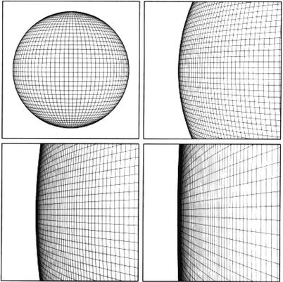
Fig. 4.21
Due to tremendous expansion during
inflation, even a universe with initial curvature will appear to be
a flat universe by the end of the inflationary phase. Source: A.H.
Guth 1998, The Inflationary
Universe, Basic Books
Inflation solves
the flatness problem as well. Due to the tremendous
expansion, any initial curvature is straightened out (see
Fig. 4.21).
Formally this can be seen as follows: during the inflationary phase
we have
 and since it is assumed that the inflationary phase lasts long
enough for the vacuum energy to be completely dominant, when it
ends we then have Ω
0 = 1. Hence the universe is flat to an extremely good
approximation.
and since it is assumed that the inflationary phase lasts long
enough for the vacuum energy to be completely dominant, when it
ends we then have Ω
0 = 1. Hence the universe is flat to an extremely good
approximation.
The inflationary model of the
very early universe predicts that today Ω 0 = 1 is valid to very
high precision; any other value of Ω 0 would require another
fine-tuning. Thus our Universe is expected to be flat.
The physical details of the inflationary scenario
are not very well known. In particular it is not yet understood how
the phase transition at the end of the inflationary phase took
place and why it did not occur earlier. But the two achievements
presented above (and some others) make an inflationary phase appear
a very plausible scenario. As we will see below (Chap. 8), the prediction of a flat universe
was recently accurately tested and it was indeed confirmed.
Furthermore, the inflationary model provides a natural, and in fact
the only plausible, explanation for the origin of density
fluctuations in the Universe which must have been present at very
early epochs as the seeds of structure formation. We will discuss
these aspects further in Chap. 7.
4.6 Problems
4.1. Big
Bang Nucleosynthesis.
1.
Calculate the baryon density at the epoch of
nucleosynthesis. How does it compare with the density in the
central regions of stars where nuclear burning takes place?
2.
It takes the Sun some ten billion years to
convert ∼ 10 % of its
hydrogen into helium, whereas in BBN, all helium is formed on a
time-scale of a minute. Can you speculate about the reasons for
this difference?
3.
During BBN, energy is released from the fusion
process. Obtain an estimate of this fusion energy generated per
unit volume, and compare it to the energy density of the photons at
the epoch of BBN. Does BBN cause a substantial heating of the
Universe?
4.2. Deceleration parameter. Assume that the
energy density of the universe is composed of N different species. Each of these
species is characterized by a density parameter Ω i and an equation-of-state
parameter w
i which
describes the relation between pressure and density, P i = w i ρ i c 2. Calculate the
deceleration parameter q
0 for this cosmological model. By specializing to the
three energy components discussed in this chapter, can you
rederive (4.35)?
4.3. The
qualitative behavior of the cosmic expansion. The general
discussion of the qualitative behavior of the solutions of the
Friedmann equation (4.33) is tedious, but some special results can
be derived quite easily. In the following, neglect the (very small)
contribution from Ω
r.
1.
For Ω
Λ = 0, show
that the universe has been expanding for all 0 < a ≤ 1, that it will continue to expand
forever in the future if Ω
m ≤ 1, and that it reaches a maximum expansion at
t max,
corresponding to the maximum scale factor a max. Calculate
a max as a
function of Ω
m.
2.
Show that the universe expands forever in the
future if Ω
Λ ≥ 0 and
Ω m ≤ 1, and
that it has been expanding in the past if 0 ≤ Ω Λ < 1, irrespective of
Ω m.
3.
For the case of a closed universe which has a
maximum expansion factor, or that of a bouncing model where a
minimum scale factor occurs, show that  ,
where t ex is
the time where the extremum of the scale factor is attained.
,
where t ex is
the time where the extremum of the scale factor is attained.
,
where t ex is
the time where the extremum of the scale factor is attained.4.4. Expansion law in a flat universe. You
will now solve the Friedmann equation (4.33) for the case of
vanishing curvature and vanishing radiation density. This describes
the model of the Universe we live in, for scale factors
a ≫ a eq.
1.
As a first step, write a = v β , and choose β such that the Friedmann equation can
be brought to the form  .
.
.2.
Then make the ansatz  , and determine
v 0 and
t a such that
the foregoing equation is solved. Note that sinh ′ (x) = cosh(x) and
, and determine
v 0 and
t a such that
the foregoing equation is solved. Note that sinh ′ (x) = cosh(x) and  .
.
, and determine
v 0 and
t a such that
the foregoing equation is solved. Note that sinh ′ (x) = cosh(x) and .3.
Combining these two steps, write the full
solution a(t) explicitly. What is the behavior of
the solution for t ≪ t a and for t ≫ t a—does it agree with your
expectations? Does this solution describe the transition from a
decelerating expansion to an accelerated one?
4.5. The
onset of inflation. Solve the Friedmann equation for a flat
universe with vanishing matter density—the situation perhaps
approximating the situation in our Universe before the end of
inflation. Use the same steps as in the previous problem to obtain
the solution. Again, there is a characteristic time scale
t a occurring in
the solution; what is the behavior of the scale factor for
t ≪ t a and for t ≫ t a? Does this correspond to
what is written in the main text for radiation dominance and vacuum
energy dominance, respectively?
4.6. Distances in cosmology. In
Sect. 4.3.3,
we quoted the expressions for the angular-diameter distance as a
function of redshift; these expressions shall be derived here.
1.
Consider a radial light ray reaching us today,
i.e., at scale factor a = 1. From the
relation (4.39), derive the relation between a small
interval da and a comoving
radial distance interval dx
along this ray.
4.7. Expansion law in an Ω Λ = 0 universe. For a model with vanishing
vacuum density, the expansion law can be obtained analytically.
1.
As preparation for the solution, we consider a
differential equation of the form

(4.84)
where C > 0 and K are constants. Solutions
of (4.84) are given in parametric form. Show by
insertion that the solution with f(t 1) = 0 reads
 for K > 0 and
0 ≤ θ ≤ 2π, and
for K > 0 and
0 ≤ θ ≤ 2π, and
 for K < 0 and
θ ≥ 0. Note that
for K < 0 and
θ ≥ 0. Note that
 .
In the special case of K = 0, show that the solution is
.
In the special case of K = 0, show that the solution is

(4.85)
(4.86)
.
In the special case of K = 0, show that the solution is
(4.87)
For the case of K > 0, show that f reaches a maximum value  at time
  , and that
f coll = 0 at
time
, and that
f coll = 0 at
time  .
.
at time , and that
f coll = 0 at
time .2.
Show that the Friedmann
equation (4.33) in the case of  is of the form (4.84), and derive the expansion law in
parametric form. Does the maximum scale factor a max that occurs for
Ω m > 1 agree
with what you found in problem 4.3? At what cosmic time
does this maximum scale factor occur? When does such a universe
recollapse?
is of the form (4.84), and derive the expansion law in
parametric form. Does the maximum scale factor a max that occurs for
Ω m > 1 agree
with what you found in problem 4.3? At what cosmic time
does this maximum scale factor occur? When does such a universe
recollapse?
is of the form (4.84), and derive the expansion law in
parametric form. Does the maximum scale factor a max that occurs for
Ω m > 1 agree
with what you found in problem 4.3? At what cosmic time
does this maximum scale factor occur? When does such a universe
recollapse?3.
As in problem 1.4, consider a sphere of mass
M and initial radius
r 0 at time
t = 0, collapsing due to
gravity. Show that the equation of motion for r(t) can be written in the
form (4.84), and determine the physical meaning of
C and K. Show that the solution derived in
problem 1.4 corresponds to the case K = 0. If the sphere at t = 0 was at rest,  , show that the sphere collapses to
point within the free-fall
time
, show that the sphere collapses to
point within the free-fall
time
 where
where  is the initial mean density of the sphere.
, show that the sphere collapses to
point within the free-fall
time
(4.88)
is the initial mean density of the sphere.4.8. The
time of return for a upward-moving object. In the text, an
analogon of a nearly flat universe has been given, namely that of
an object shot vertically upwards from the surface of the Earth.
The time at which it returns to the surface is either ‘short’, or
the velocity has to be very well fine-tuned. Using the parametric
solution of the equation of motion derived in the previous
exercise, we can now consider this situation quantitatively.
1.
Show that the equation of motion for the object
can be written in the form  , where
M E is the mass
of the Earth. Relate the integration constant K to the initial velocity v 0 of the object, and
assume in the following that v 0 < v esc, where
, where
M E is the mass
of the Earth. Relate the integration constant K to the initial velocity v 0 of the object, and
assume in the following that v 0 < v esc, where  ,
with r
E ≈ 6380 km being the Earth’s radius.
,
with r
E ≈ 6380 km being the Earth’s radius.
, where
M E is the mass
of the Earth. Relate the integration constant K to the initial velocity v 0 of the object, and
assume in the following that v 0 < v esc, where ,
with r
E ≈ 6380 km being the Earth’s radius.2.
From the parametric solution of the last problem,
calculate the time t
ret at which the object returns to the Earth surface.
For this, you can assume that the time-of-flight is ‘long’, i.e.,
much longer than r
E∕v
0. Then find the relation between K and the time t ret.
3.
Combining the last two steps, obtain the relation
between the initial velocity v 0 and the time of return
t ret. What
fraction of the escape velocity does the object have to have
initially if it should return after 1 day (1 year)?
4.9. Baryon cooling in the Universe. Suppose
that at some epoch after recombination, the baryons are fully
decoupled from the photons, so that there is no energy transfer
from one species to the other. Use (4.47) to derive the
expected redshift dependence of the baryon temperature during this
epoch.
4.10. Thermal velocity of the cosmic neutrino
background. Using (4.47), calculate the current characteristic
velocity of neutrinos that decoupled in the early phase of the Big
Bang.
4.11. Some properties of the Einstein–de Sitter
model. Consider the Einstein–de Sitter model.
1.
Calculate the look-back time τ(z). At what redshift was the age of the
Universe half of its current age?
2.
What is the volume of the spherical shell between
redshifts z and
z +Δ z?
3.
Assume the comoving density n com of a class of cosmic
objects is constant; how many of these are contained in sphere
around us with maximum redshift z? Check that your result agrees with
the expected one for z ≪ 1.
Footnotes
2
Returning to the picture of the raisins in a
yeast dough above: On the one hand, the raisins have a velocity
relative to each other, and thus are ‘moving’. On the other hand,
they are stuck in the dough, and thus have no (peculiar)
velocity—they are comoving with the dough. Their mutual relative
velocity thus results solely from the expansion of the dough, which
can be considered an analog to the expanding spacetime.
3
In the original notation, the Λ used here is denoted by Λ c 2; for notational
simplicity, we absorb the c
2 into the definition of Λ.
4
The notation ‘dust’ should not be confused with
the dust that is responsible for the extinction and reddening of
light—‘dust’ in cosmology only denotes matter with P = 0.
5
In the literature, different definitions for
Ω 0 are used.
Often the notation Ω
0 is used for Ω
m.
6
The surface of a cylinder is also considered a
flat space, like a plane, because the sum of angles in a triangle
on a cylinder is also 180∘. But the surface of a
cylinder obviously has a topology different from a plane; in
particular, closed straight lines do exist—walking on a cylinder in
a direction perpendicular to its axis, one will return to the
starting point after a finite amount of time.
7
Generally, it can be shown that the specific
intensity I
ν changes due to
redshift according to
 Here, I ν is the specific intensity today
at frequency ν and
Here, I ν is the specific intensity today
at frequency ν and
 is the specific
intensity at redshift z at
frequency
is the specific
intensity at redshift z at
frequency  .
.
(4.46)
is the specific
intensity at redshift z at
frequency .8
Compare this energy density with that of a
blackbody photon distribution; they are the same except for the
prefactor. This prefactor is determined by the number of bosonic
and fermionic particle species which are relativistic at
temperature T.
9
The total number of photons emitted during
stellar evolution is negligible compared to the number of CMB
photons.
10
For their research in the field of Solar
neutrinos, Raymond Davis and Masatoshi Koshiba were awarded with
one half of the Nobel Prize in Physics in 2002. The other half was
awarded to Ricardo Giacconi for his pioneering work in the field of
X-ray astronomy.
11
From the fundamental constants G, c and h P, one can form a unique
combination with the dimension of a mass,  ,
called the Planck mass. This is the mass scale where one expects
that General Relativity ceases to be valid and that it has to be
generalized to a quantum theory of gravity. Up to now, no plausible
model for such a quantum gravity has been found.
,
called the Planck mass. This is the mass scale where one expects
that General Relativity ceases to be valid and that it has to be
generalized to a quantum theory of gravity. Up to now, no plausible
model for such a quantum gravity has been found.
,
called the Planck mass. This is the mass scale where one expects
that General Relativity ceases to be valid and that it has to be
generalized to a quantum theory of gravity. Up to now, no plausible
model for such a quantum gravity has been found.12
One might be surprised about the assumption that
a particle of such high mass should be stable—given that there are
only very few particles known to be stable, and they all have very
small mass—the heaviest one being the proton. The Standard Model
predicts that the baryon number is a conserved quantity, i.e., one
cannot change the net number of baryons. For example, in creating a
proton–antiproton pair, the net baryon number is changed by
 ;
in the decay of the free neutron, baryon number is conserved as
well. Since the proton is the lightest baryon, there is no particle
into which it can decay without violating baryon
conservation—that’s why we believe the proton is stable. If such a
conserved quantity exists in the extended model of elementary
particles (for example, in supersymmetry there is a so-called
R-parity), then the lightest of the particles which ‘carries’ this
quantity must be stable as well.
;
in the decay of the free neutron, baryon number is conserved as
well. Since the proton is the lightest baryon, there is no particle
into which it can decay without violating baryon
conservation—that’s why we believe the proton is stable. If such a
conserved quantity exists in the extended model of elementary
particles (for example, in supersymmetry there is a so-called
R-parity), then the lightest of the particles which ‘carries’ this
quantity must be stable as well.13
The recombination of hydrogen—and also that of
helium which occurred at slightly higher redshifts—perturbed the
exact Planck shape of the photon distribution, adding to it the
Lyman-alpha photons and the photon pairs from the two-photon
transition. This slight perturbation in the CMB spectrum should in
principle still be present today. Unfortunately, it lies in a
wavelength range ( ∼ 200 μm) where the dust emission from the
Galaxy is very strong; in addition, the wavelength range coincides
with the peak of the far-infrared background radiation (see
Sect. 9.5.1). Therefore, the detection of
this spectral distortion will be extremely difficult.
14
For instance, there exists a cosmic X-ray
background (CXB; see Sect. 9.5) which is radiation that
appeared isotropic in early measurements. For a long time, a
possible explanation for this was suggested to be a hot
intergalactic medium with temperature of  emitting
bremsstrahlung radiation. But such a hot intergalactic gas would
modify the spectrum of the CMB via the scattering of CMB photons to
higher frequencies by energetic electrons (inverse Compton
scattering). This explanation for the source of the CXB was
excluded by the COBE measurements. From observations by the X-ray
satellites ROSAT, Chandra, and XMM-Newton, with their high angular
resolution, we know today that the CXB is a superposition of
radiation from discrete sources, mostly AGNs.
emitting
bremsstrahlung radiation. But such a hot intergalactic gas would
modify the spectrum of the CMB via the scattering of CMB photons to
higher frequencies by energetic electrons (inverse Compton
scattering). This explanation for the source of the CXB was
excluded by the COBE measurements. From observations by the X-ray
satellites ROSAT, Chandra, and XMM-Newton, with their high angular
resolution, we know today that the CXB is a superposition of
radiation from discrete sources, mostly AGNs.15
We ignore peculiar motions here which may cause
an additional (Doppler-)redshift. These are typically  and are thus small
compared to cosmological redshifts.
and are thus small
compared to cosmological redshifts.
and are thus small
compared to cosmological redshifts.