Galaxies are not uniformly distributed in space,
but instead show a tendency to gather together in galaxy groups and clusters of galaxies. This effect can
be clearly recognized in the projection of bright galaxies on the
sky (see Figs. 6.1 and 6.2). The Milky Way itself is a member of a
group, called the Local Group (Sect. 6.1), which implies that
we are living in a locally overdense region of the Universe.
The transition between groups and clusters of
galaxies is smooth. Historically, the distinction was made on the
basis of the number of their member galaxies. Roughly speaking, an
accumulation of galaxies is called a group if it consists of
 members within a sphere of diameter
  . Clusters have
 members and diameters
  . A formal
definition of a cluster is presented further below. An example of a
group and a cluster of galaxies is displayed in Fig. 6.3.
. A formal
definition of a cluster is presented further below. An example of a
group and a cluster of galaxies is displayed in Fig. 6.3.
members within a sphere of diameter . Clusters have
members and diameters . A formal
definition of a cluster is presented further below. An example of a
group and a cluster of galaxies is displayed in Fig. 6.3.Clusters of galaxies are very massive: typical
values are  for massive
clusters, whereas for groups
for massive
clusters, whereas for groups  is
characteristic, with the total mass range of groups and clusters
extending over
is
characteristic, with the total mass range of groups and clusters
extending over  .
.
for massive
clusters, whereas for groups is
characteristic, with the total mass range of groups and clusters
extending over .Originally, clusters of galaxies were
characterized as such by the observed spatial concentration of
galaxies. Today we know that, although the galaxies determine the
optical appearance of a cluster, the mass contained in galaxies
contributes only a small fraction to the total mass of a cluster.
Through advances in X-ray astronomy, it was discovered that galaxy
clusters are intense sources of X-ray radiation which is emitted by
a hot gas (T ∼ 3 ×
107 K) located between the galaxies. This intergalactic
gas (intracluster medium,
ICM) contains more baryons than the stars seen in the member
galaxies. From the dynamics of galaxies, from the properties of the
intracluster gas, and from the gravitational lens effect we deduce
the existence of dark matter in galaxy clusters, dominating the
cluster mass like it does for galaxies.
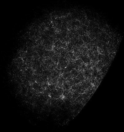
Fig. 6.1
The distribution of galaxies in the
Northern sky, as compiled in the Lick catalog. This catalog
contains the galaxy number counts for ‘pixels’ of 10
′ × 10
′ each. It is
clearly seen that the distribution of galaxies on the sphere is far
from being homogeneous. Instead it is distinctly structured. For an
all-sky map of bright galaxies, as observed at near-IR wavelengths,
see Fig. 1.52. Source: Webpage E.J. Groth,
Princeton University; adapted from M. Seldner et al. 1977,
New reduction of the Lick catalog
of galaxies, AJ 82, 249
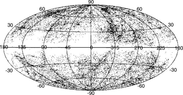
Fig. 6.2
The distribution of all galaxies brighter
than B < 14. 5 on the
sphere, plotted in Galactic coordinates. The Zone of Avoidance is
clearly seen as the region near the Galactic plane. Source: N.A.
Sharp 1986, The whole-sky
distribution of galaxies, PASP 98, 740, p. 753,
Fig. 14
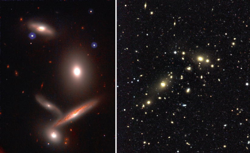
Fig. 6.3
The left
panel shows HCG40, a compact group of galaxies, observed
with the Subaru telescope on Mauna-Kea. The right panel displays the cluster of
galaxies Cl 0053−37, observed with the WFI at the ESO/MPG
2.2-m telescope. Credits: Left: Copyright @ Subaru Telescope,
NAOJ. All rights reserved. Right: M. Schirmer, European Southern
Observatory
Clusters of galaxies play a very important role
in observational cosmology. They are the most massive bound and
relaxed (i.e., in a state of approximate dynamical equilibrium)
cosmic structures, and therefore mark the most prominent density
peaks of the large-scale structure in the Universe. For that
reason, their cosmological evolution is directly related to the
growth of cosmic structures, as will be discussed in
Chaps. 7 and 8. Due to their high galaxy number
density, clusters and groups are also ideal laboratories for
studying interactions between galaxies and their effect on the
galaxy population. For instance, the fact that elliptical galaxies
are preferentially found in clusters indicates the impact of the
local galaxy density on the morphology and evolution of
galaxies.
Outline of this
chapter.We will start be discussing the nearest association
of galaxies, namely the Local Group, of which the Milky Way is a
member. In Sect. 6.2, we describe the identification of galaxy
clusters with optical methods, and some of the resulting cluster
and group catalogs. The spatial distribution of galaxies in
clusters and their dynamics will be studied in Sect. 6.3. We will show that
the relative motion of galaxies in clusters implies a much higher
cluster mass than can be accounted for by the stars seen in the
member galaxies. Whereas not all stars are bound in individual
cluster galaxies, but some are distributed throughout the cluster,
forming the intracluster light component, this additional stellar
component only constitutes a ∼ 20 % contribution to the overall
stellar mass budget.
The space between the galaxies is filled by a hot
gas, detected by its X-ray emission and its impact on the spectrum
of the observed cosmic microwave background radiation seen in the
direction of clusters. We study this intracluster medium in
Sect. 6.4; in
particular we show how the properties of the gas can be used for
mass determination of clusters. These mass estimates are in good
agreement with those obtained from the dynamics of galaxies,
reinforcing the conclusion the clusters contain more mass than
directly observed, even if the mass of the hot gas is taken into
account. The central galaxies of many clusters contain an AGN,
whose energy output has a distinct impact on the properties of the
hot gas.
In Sect. 6.5 we show that there exist tight relations
between the temperature of the hot intracluster gas, its X-ray and
optical/near-IR luminosities, the galaxy velocity dispersion and
the cluster mass. These scaling relations, analogous to the scaling
relations of galaxies, indicate that clusters of the same mass have
rather similar properties.
Clusters of galaxies can act as gravitational
lenses, giving rise to spectacular imaging phenomena. Those will be
discussed in Sect. 6.6, together with a method which allows one to
obtain maps of the total matter distribution in clusters. In
particular, gravitational lensing yields a third, fully independent
method for determining cluster masses. We will find that more than
80 % of the cluster mass is made of dark matter, only ∼ 3 % of
stars, and some 15 % of the baryons in the intracluster
medium.
The dense environment of groups and clusters may
affect the evolution of their member galaxies; we shall therefore
discuss the galaxy population of clusters in Sect. 6.7; more generally, we
will describe the properties of galaxies in relation to the density
of their environment. Finally, we discuss in Sect. 6.8 some evolutionary
aspects of the cluster population.
6.1 The Local Group
The Milky Way is a member of the Local Group. Within a distance
of ∼ 1 Mpc around our Galaxy, about 35 galaxies were known at the
turn of the Millennium; these ‘classical’ Local Group members are
listed in Table 6.1, and a sketch of their spatial distribution
is given in Fig. 6.4. With the Sloan Digital Sky Survey (SDSS;
see Sect. 1.4), about 20 additional very faint
galaxies in the Local Group have been found. Most of them cannot be
detected solely as overdensity of stars on the sky, because their
density contrast is too low. However, by filtering the star catalog
according to stellar colors and magnitudes, which together allow
for the selection of stars from an old population at similar
distances, spatial overdensities can be identified. We will return
to them in Sect. 7.8.
6.1.1 Phenomenology
The Milky Way (MW), M31 (Andromeda; see
Fig. 6.5), and
M33 (Fig. 6.6)
are the three spiral galaxies in the Local Group, and they are also
its most luminous members. The Andromeda galaxy is located at a
distance of 770 kpc from us, M33 at about 850 kpc. The Local Group
member next in luminosity is the Large Magellanic Cloud (LMC, see
Fig. 6.7),
which is orbiting around the Milky Way, together with the Small
Magellanic Cloud (SMC), at a distance of ∼ 50 kpc ( ∼ 60 kpc,
respectively, for the SMC). Both are satellite galaxies of the
Milky Way and belong to the class of irregular galaxies (like about
11 other Local Group members). The other members of the Local Group
are dwarf galaxies, which are very small and faint (see
Fig. 6.8 for
three examples). Because of their low luminosity and their low
surface brightness, many of the known members of the Local Group
were detected only fairly recently. For example, the Antlia galaxy,
a dwarf spheroidal galaxy, was found in 1997. Its luminosity is
about 104 times smaller than that of the Milky
Way.
Table 6.1
‘Classical’ members of the Local
Group
|
Galaxy
|
Type
|
M
B
|
RA/dec.
|
ℓ,b
|
D(kpc)
|
v
r (km/s)
|
|---|---|---|---|---|---|---|
|
Milky Way
|
Sbc I-II
|
− 20. 0
|
1830 − 30
|
0, 0
|
8
|
0
|
|
LMC
|
Ir III-IV
|
− 18. 5
|
0524 − 60
|
280, − 33
|
50
|
270
|
|
SMC
|
Ir IV-V
|
− 17. 1
|
0051 − 73
|
303, − 44
|
63
|
163
|
|
Sgr I
|
dSph?
|
1856 − 30
|
6, − 14
|
20
|
140
|
|
|
Fornax
|
dE0
|
− 12. 0
|
0237 − 34
|
237, − 65
|
138
|
55
|
|
Sculptor Dwarf
|
dSph
|
− 9. 8
|
0057 − 33
|
286, − 84
|
88
|
110
|
|
Leo I
|
dSph
|
− 11. 9
|
1005 + 12
|
226, +49
|
790
|
168
|
|
Leo II
|
dSph
|
− 10. 1
|
1110 + 22
|
220, +67
|
205
|
90
|
|
Ursa Minor
|
dSph
|
− 8. 9
|
1508 + 67
|
105, +45
|
69
|
− 209
|
|
Draco
|
dSph
|
− 9. 4
|
1719 + 58
|
86, +35
|
79
|
− 281
|
|
Carina
|
dSph
|
− 9. 4
|
0640 − 50
|
260, − 22
|
94
|
229
|
|
Sextans
|
dSph
|
− 9. 5
|
1010 − 01
|
243, +42
|
86
|
230
|
|
M31
|
Sb I-II
|
− 21. 2
|
0040 + 41
|
121, − 22
|
770
|
− 297
|
|
M32 = NGC 221
|
dE2
|
− 16. 5
|
0039 + 40
|
121, − 22
|
730
|
− 200
|
|
M110 = NGC 205
|
dE5p
|
− 16. 4
|
0037 + 41
|
121, − 21
|
730
|
− 239
|
|
NGC 185
|
dE3p
|
− 15. 6
|
0036 + 48
|
121, − 14
|
620
|
− 202
|
|
NGC 147
|
dE5
|
− 15. 1
|
0030 + 48
|
120, − 14
|
755
|
− 193
|
|
And I
|
dSph
|
− 11. 8
|
0043 + 37
|
122, − 25
|
790
|
–
|
|
And II
|
dSph
|
− 11. 8
|
0113 + 33
|
129, − 29
|
680
|
–
|
|
And III
|
dSph
|
− 10. 2
|
0032 + 36
|
119, − 26
|
760
|
–
|
|
Cas = And VII
|
dSph
|
2326 + 50
|
109, − 09
|
690
|
–
|
|
|
Peg = DDO 216
|
dIr/dSph
|
− 12. 9
|
2328 + 14
|
94, − 43
|
760
|
–
|
|
Peg II = And VI
|
dSph
|
− 11. 3
|
2351 + 24
|
106, − 36
|
775
|
–
|
|
LGS 3
|
dIr/dSph
|
− 9. 8
|
0101 + 21
|
126, − 41
|
620
|
− 277
|
|
M33
|
Sc II-III
|
− 18. 9
|
0131 + 30
|
134, − 31
|
850
|
− 179
|
|
NGC 6822
|
dIr IV-V
|
− 16. 0
|
1942 − 15
|
025, − 18
|
500
|
− 57
|
|
IC 1613
|
dIr V
|
− 15. 3
|
0102 + 01
|
130, − 60
|
715
|
− 234
|
|
Sagittarius
|
dIr V
|
− 12. 0
|
1927 − 17
|
21, +16
|
1060
|
− 79
|
|
WLM
|
dIr IV-V
|
− 14. 4
|
2359 − 15
|
76, − 74
|
945
|
− 116
|
|
IC 10
|
dIr IV
|
− 16. 0
|
0017 + 59
|
119, − 03
|
660
|
− 344
|
|
DDO 210, Aqr
|
dIr/dSph
|
− 10. 9
|
2044 − 13
|
34, − 31
|
950
|
− 137
|
|
Phoenix Dwarf
|
dIr/dSph
|
− 9. 8
|
0149 − 44
|
272, 68
|
405
|
56
|
|
Tucana
|
dSph
|
− 9. 6
|
2241 − 64
|
323, − 48
|
870
|
–
|
|
Leo A = DDO 69
|
dIr V
|
− 11. 7
|
0959 + 30
|
196, 52
|
800
|
–
|
|
Cetus Dwarf
|
dSph
|
− 10. 1
|
0026 − 11
|
101, − 72
|
775
|
–
|
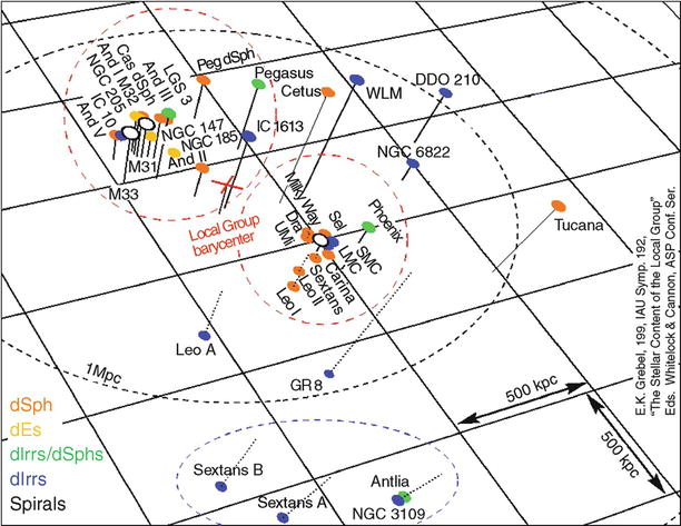
Fig. 6.4
Schematic distribution of galaxies in the
Local Group, with the Milky Way at the center of the figure Shown
are only the ‘classical’ Local Group members which were known
before 2000; most of the newly found galaxies in the Local Group
are ultra-faint dwarfs. Credit: E. Grebel, Astronomical Institute,
University of Basel, Switzerland
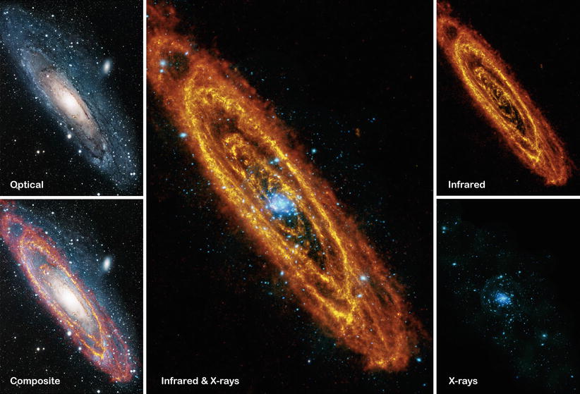
Fig. 6.5
M31, the Andromeda galaxy, seen in
different wavelengths. All images show a region of
1. 5∘× 2∘. Compared to the optical image
(top left) which shows the
stellar distribution of the galaxy, the far-infrared emission shown
on the top right displays
predominantly the dust component of the interstellar medium. Heated
by young massive stars, the dust re-radiates the absorbed energy at
long wavelengths, here shown with a 250 μm exposure taken with the
Herschel Observatory. The X-ray image (bottom right), taken with XMM-Newton,
mainly displays the distribution of X-ray binaries and supernova
remnants; in particular the former are much more concentrated
towards the central parts of the galaxy. The two composite images
in the center and
bottom left compare the
distributions of the various components of M31. Credit &
Copyright: infrared: ESA/Herschel/PACS/SPIRE/J. Fritz, U. Gent;
X-ray: ESA/XMM-Newton/EPIC/W. Pietsch, MPE; optical: R.
Gendler
Many of the dwarf galaxies are grouped around the
Galaxy or around M31; these are known as satellite galaxies. Distributed around
the Milky Way are the LMC, the SMC, and about 20 dwarf galaxies,
several of them in the so-called Magellanic Stream (see
Fig. 2.19), a long, extended band of
neutral hydrogen which was stripped from the Magellanic Clouds
about 2 × 10⁸ yr ago by tidal interactions with the
Milky Way. The Magellanic Stream contains about 3 × 10⁸
M ⊙ of neutral
hydrogen.
The spatial distribution of satellite galaxies
around the Milky Way shows a pronounced peculiarity, in that the 11
closest satellites form a highly flattened system. These satellites
appear to lie essentially in a plane which is oriented
perpendicular to the Galactic plane, concentrated along the minor
axis of the disk. The satellites around M31 also seem to be
distributed in an anisotropic way around their host. In fact,
satellite galaxies around spirals seem to be preferentially located
near the short axes of the projected light distribution, which has
been termed the Holmberg effect, although the statistical
significance of this alignment has been questioned, in particular
in recent years. We will come back to this issue in
Sect. 7.8.
In fact, the Local Group is not a group of
galaxies in the sense of this chapter; its spatial extent is too
large for a group of this mass, and it is not dynamically relaxed.
The bimodal distribution of galaxies in the Local Group seen in
Fig. 6.4
instead suggests that two small galaxy groups—one centered on M31,
the other one centered on the Milky Way—are in a process of
merging.
6.1.2 Mass estimate
We will present a simple mass estimate of the
Local Group, from which we will find that it is considerably more
massive than one would conclude from the observed luminosity of the
associated galaxies.
M31 is one of the very few galaxies with a
blueshifted spectrum. Hence, Andromeda and the Milky Way are
approaching each other, at a relative velocity of v ≈ 120 km∕s. This value results from
the velocity of M31 relative to the Sun of v ≈ 300 km∕s, and from the motion of
the Sun around the Galactic center. Together with the distance to
M31 of D ∼ 770 kpc, we
conclude that both galaxies will collide on a time-scale of ∼ 6 ×
109 yr, if we disregard the transverse component of the
relative velocity. From measurements of the proper motion of M31,
one finds that its transverse velocity is small—thus a collision
with the Milky Way will almost certainly occur.
The luminosity of the Local Group is dominated by
the Milky Way and by M31, which together produce about 90 % of the
total luminosity. If the mass density follows the light
distribution, the dynamics of the Local Group should also be
dominated by these two galaxies. Therefore, one can try to estimate
the mass of the two galaxies from their relative motion, and with
this also the mass of the Local Group.
In the early phases of the Universe, the Galaxy
and M31 were close together and both took part in the Hubble
expansion. By their mutual gravitational attraction, their relative
motion was decelerated until it came to a halt—at a time
t max at which
the two galaxies had their maximum separation r max from each other. From
this time on, they have been moving towards each other. The
relative velocity v(t) and the separation r(t) follow from the conservation of
energy,
 where M is the sum of the
masses of the Milky Way and M31, and C is an integration constant, related
to the total energy of the M31/MW-system. This constant can be
determined by considering (6.1) at the time of maximum separation, when
r = r max and v = 0. With this,
where M is the sum of the
masses of the Milky Way and M31, and C is an integration constant, related
to the total energy of the M31/MW-system. This constant can be
determined by considering (6.1) at the time of maximum separation, when
r = r max and v = 0. With this,
 follows immediately. Since
  , (6.1) is a differential
equation for r(t),
, (6.1) is a differential
equation for r(t),

(6.1)
, (6.1) is a differential
equation for r(t),
It can be solved using the initial condition
r = 0 at t = 0. For our purpose, an approximate
consideration is sufficient. Solving the equation for dt we obtain, by integration, a relation
between r max
and t max,
 Since the differential equation is symmetric with respect to
changing v → −v, the collision will happen at
2t max.
Estimating the time from today to the collision, by assuming the
relative velocity to be constant during this time, then yields
Since the differential equation is symmetric with respect to
changing v → −v, the collision will happen at
2t max.
Estimating the time from today to the collision, by assuming the
relative velocity to be constant during this time, then yields
 ,
and one obtains
,
and one obtains  , or
, or
 where t 0 ≈ 14 ×
109 yr is the current age of the Universe. Hence,
together with (6.2) this yields
where t 0 ≈ 14 ×
109 yr is the current age of the Universe. Hence,
together with (6.2) this yields
 Now by inserting the values r(t 0) = D and v = v(t 0), we obtain the mass
M,
Now by inserting the values r(t 0) = D and v = v(t 0), we obtain the mass
M,
 This mass is much larger than the mass of the two galaxies as
observed in stars and gas. The mass estimate yields a mass-to-light
ratio for the Local Group of
This mass is much larger than the mass of the two galaxies as
observed in stars and gas. The mass estimate yields a mass-to-light
ratio for the Local Group of  , much larger
than that of any known stellar population. This is therefore
another indication of the presence of dark matter because we can
see only about 5 % of the estimated mass in the Milky Way and
Andromeda. Another mass estimate follows from the kinematics of the
Magellanic Stream, which also yields
, much larger
than that of any known stellar population. This is therefore
another indication of the presence of dark matter because we can
see only about 5 % of the estimated mass in the Milky Way and
Andromeda. Another mass estimate follows from the kinematics of the
Magellanic Stream, which also yields  .
.
(6.2)
,
and one obtains , or
(6.3)
(6.4)
(6.5)
, much larger
than that of any known stellar population. This is therefore
another indication of the presence of dark matter because we can
see only about 5 % of the estimated mass in the Milky Way and
Andromeda. Another mass estimate follows from the kinematics of the
Magellanic Stream, which also yields .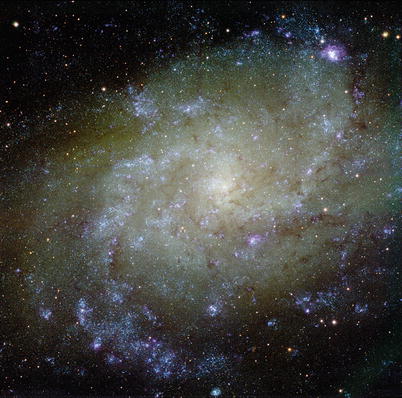
Fig. 6.6
Multi-band (u,g,r) composite image of the
Triangulum Galaxy (M33), a Local Group spiral with an estimated
distance of ∼ 850 kpc. With its visible diameter of ∼ 15 kpc, it is
the third largest galaxy of the Local Group; its stellar mass is
about 1/10 that of the Milky Way. Observations of water masers in
this galaxy enabled the measurement of its proper motion,
indicating that it is heading towards M31. The bluish emission is
due to regions of active star formation; indeed, the bright region
near the top-right of the images is one of the most luminous
Hii regions known. This
is the first image taken with the wide-field camera of the new 2-m
Fraunhofer telescope on the Wendelstein Observatory and covers 30
′ on a side.
Credit: Wendelstein Observatory, Universitätssternwarte der
Ludwig-Maximilians-Universität München
6.1.3 Other components of the Local Group
Tidal
streams. One of the most interesting galaxies in the Local
Group is the Sagittarius dwarf
galaxy which was only discovered in 1994. Since it is
located in the direction of the Galactic bulge, it is barely
visible on optical images, if at all, as an overdensity of stars.
Furthermore, it has a very low surface brightness. It was
discovered in an analysis of stellar kinematics in the direction of
the bulge, in which a coherent group of stars was found with a
velocity distinctly different from that of bulge stars. In
addition, the stars belonging to this overdensity have a much lower
metallicity, reflected in their colors. The Sagittarius dwarf
galaxy is located close to the Galactic plane, at a distance of
about 16 kpc from the Galactic center and nearly in the direct
extension of our line-of-sight to the GC. This proximity implies
that it must be experiencing strong tidal gravitational forces on
its orbit around the Milky Way; over the course of time, these will
have the effect that the Sagittarius dwarf galaxy will be slowly
disrupted. In fact, in recent years a relatively narrow band of
stars was found around the Milky Way. These stars are located along
the orbit of the Sagittarius galaxy (see Fig. 2.18). Their chemical composition
supports the interpretation that they are stars stripped from the
Sagittarius dwarf galaxy by tidal forces. In addition, globular
clusters were identified which presumably once belonged to the
Sagittarius dwarf galaxy, but which were also removed from it by
tidal forces and are now part of the globular cluster population in
the Galactic halo. Indeed, more tidal streams have been discovered
recently, both in the Milky Way and in Andromeda, as well as in
other neighboring galaxies.
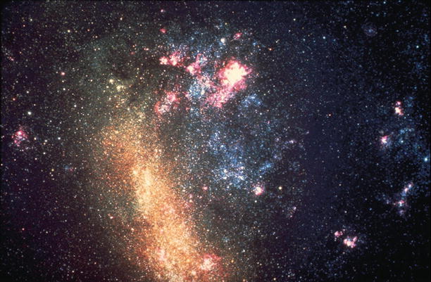
Fig. 6.7
An image of the Large Magellanic Cloud
(LMC), taken with the CTIO 4-m telescope. Credit & Copyright:
AURA/NOAO/NSF
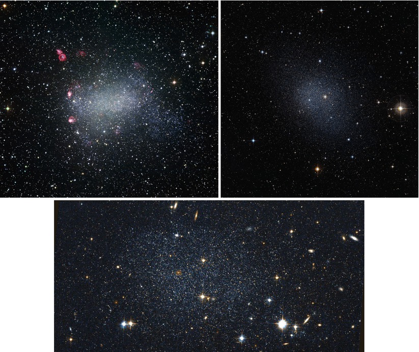
Fig. 6.8
Upper
left: NGC 6822, also known as Barnard’s Galaxy, is one of
the dwarf elliptical galaxies of the Local Group, located at a
distance of 500 kpc from the Milky Way. This color composite image
covers a region of 34 ′ on the side, and was taken with
the WFI@ESO/MPG 2.2 m telescope on La Silla. The reddish nebulae in
the image indicate regions of active star formation. Upper right: The Fornax dwarf
spheroidal galaxy is a satellite of the Milky Way, at a distance of
140 kpc. The image size is about 17 ′ × 13 ′ , and was extracted from the
Digitized Sky Survey II. Bottom: The Antlia dwarf galaxy lies at
a distance of 1. 3 Mpc, at the edge of the Local Group. This
color-composite HST images covers 3.′2 ×
1.′5. Credit: Top
left: ESO; Top
right: ESO/Digitized Sky Survey 2; Bottom: ESA/NASA
The neighborhood
of the Local Group. The Local Group is indeed a
concentration of galaxies: while it contains more than 50 members
within ∼ 1 Mpc, the next neighboring galaxies are found only in the
Sculptor Group, which contains about six members1 and is located at a distance of
D ∼ 1. 8 Mpc. The next
galaxy group after this is the M81-group of ∼ 8 galaxies at
D ∼ 3. 1 Mpc, the two most
prominent galaxies of which are displayed in Fig. 6.9.
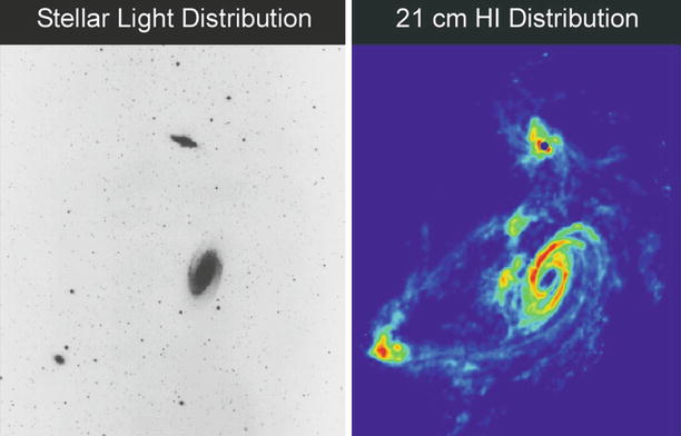
Fig. 6.9
The left
panel shows an optical image of the galaxies M81
(bottom) and M82
(top), two members of the
M81-group, about 3. 1 Mpc away (see also Fig. 1.3 for a detailed view of M82).
These two galaxies are moving around each other, and the
gravitational interaction taking place, as clearly seen in the
distribution of atomic hydrogen (right panel) which has been stripped
off the galaxies due to gravitational interactions, may be the
reason for the violent star formation in M82. M82 is an
archetypical starburst galaxy. Credit: Image courtesy of National
Radio Astronomy Observatory/AUI
The other nearby associations of galaxies within
10 Mpc from us shall also be mentioned: the Centaurus group with 17
members and D ∼ 3. 5 Mpc,
the M101-group with 5 members and D ∼ 7. 7 Mpc, the M66- and M96-group
with together 10 members located at D ∼ 9. 4 Mpc, and the NGC 1023-group
with 6 members at D = 9. 6 Mpc.
Most galaxies are members of a group. Many more
dwarf galaxies exist than luminous galaxies, and dwarf galaxies are
located preferentially in the vicinity of larger galaxies. Some
members of the Local Group are so under-luminous that they would
hardly be observable outside the Local Group.
One large concentration of galaxies was already
known in the eighteenth century (W. Herschel)—the Virgo cluster. Its galaxies extend over
a region of about 10∘× 10∘ in the sky, and
its distance is D ∼ 16 Mpc.
The Virgo cluster consists of about 250 large galaxies and more
than 2000 smaller ones; the central galaxy of the cluster is the
radio galaxy M87 (Fig. 1.11). In the classification scheme
of galaxy clusters, Virgo is considered an irregular cluster. The
closest regular massive galaxy cluster is the Coma cluster (see Fig. 1.17), at a distance of about
D ∼ 90 Mpc.
6.2 Optical cluster searches
6.2.1 The Abell catalog
George Abell compiled a catalog of galaxy
clusters, published in 1958, in which he identified regions in the
sky that show an overdensity of galaxies. This identification was
performed by eye on photoplates from the Palomar Observatory Sky Survey (POSS),
a photographic atlas of the Northern (δ > −30∘) sky (see
Sect. 1.4). He omitted the Galactic disk
region because the observation of galaxies is considerably more
problematic there, due to extinction and the high stellar density
(see also Fig. 6.2).
Abell’s criteria
and his catalog. The criteria Abell applied for the
identification of clusters refer to an overdensity of galaxies
within a specified solid angle. According to these criteria, a
cluster contains ≥ 50 galaxies in a magnitude interval m 3 ≤ m ≤ m 3 + 2, where m 3 is the apparent
magnitude of the third brightest galaxy in the cluster.2 These galaxies must be
located within a circle of angular radius

(6.6)
where z
is the estimated redshift. The latter is estimated by the
assumption that the luminosity of the tenth brightest galaxy in a
cluster is the same for all clusters. A calibration of this
distance estimate is performed on clusters of known redshift.
θ A is called
the Abell radius of a
cluster, and corresponds to a physical radius of R A ≈ 1. 5h −1 Mpc.
The so-determined redshift should be within the
range 0. 02 ≤ z ≤ 0. 2 for
the selection of Abell clusters. The lower limit is chosen such
that a cluster can be found on a single POSS photoplate
( ∼ 6∘× 6∘) and does not extend over several
plates, which would make the search more difficult, e.g., because
the photographic sensitivity may differ for individual plates. The
upper redshift bound is chosen due to the sensitivity limit of the
photoplates.
The Abell catalog contains 1682 clusters which
all fulfill the above criteria. In addition, it lists 1030 clusters
that were found in the search, but which do not fulfill all of the
criteria (most of these contain between 30 and 49 galaxies). An
extension of the catalog to the Southern sky was published by
Abell, Corwin & Olowin in 1989. This ACO catalog contains 4076
clusters, including the members of the original catalog. Another
important catalog of galaxy clusters is the Zwicky catalog
(1961–1968), which contains more clusters, but which is considered
less reliable, since the applied selection criteria resulted in
more spurious cluster candidates than is the case for the Abell
catalog.
Problems in the
optical search for clusters. The selection of galaxy
clusters from an overdensity of galaxies on the sphere is not
without problems, in particular if these catalogs are to be used
for statistical purposes. An ideal catalog ought to fulfill two
criteria: first it should be complete, in the sense that all
objects which fulfill the selection criteria are contained in the
catalog. Second it should be pure (often also called ‘reliable’),
i.e., it should not contain any objects that do not belong in the
catalog because they do not fulfill the criteria (so-called false
positives). The Abell catalog is neither complete, nor is it pure.
We will briefly discuss why completeness and reliability cannot be
expected in a catalog compiled in this way.
A galaxy cluster is a three-dimensional object,
whereas galaxy counts on images are necessarily based on the
projection of galaxy positions onto the sky. Therefore, projection
effects are inevitable. Random overdensities on the sphere caused
by line-of-sight projection may easily be classified as clusters.
The reverse effect is likewise possible: due to fluctuations in the
number density of foreground galaxies, a cluster at high redshift
may be classified as an insignificant fluctuation—and thus remain
undiscovered.
Of course, not all members of a cluster
classified as such are in fact galaxies in the cluster, as here
projection effects also play an important role. Furthermore, the
redshift estimate is relatively coarse. In the meantime,
spectroscopic analyses have been performed for many of the Abell
clusters, and it has been found that Abell’s redshift estimates
have an error of about 30 %—they are surprisingly accurate,
considering the coarseness of his assumptions.
The Abell catalog is based on visual inspection
of photographic plates. It is therefore partly subjective. Today,
the Abell criteria can be applied to digitized images in an
objective manner, using automated searches. From these, it was
found that the results are not much different. The visual search
thus was performed with great care and has to be recognized as a
great accomplishment. For this reason, and in spite of the
potential problems discussed above, the Abell and the ACO catalogs
are still frequently used.
The clusters in the catalog are ordered by right
ascension and are numbered. For example, Abell 851 is the 851st
entry in the catalog, also denoted as A851. With a redshift of
z = 0. 41, A851 is the most
distant Abell cluster.
Abell
classes. The Abell and ACO catalogs divide clusters into
so-called richness and distance classes. Table 6.2 lists the criteria for
the richness classes, while Table 6.3 lists those for the
distance classes, with the number of clusters in each class
referring to the original Abell catalog (i.e., without the ACO
extension).
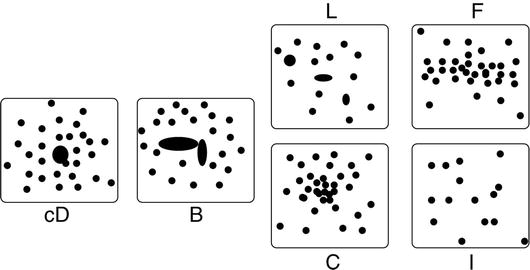
Fig. 6.10
Rough morphological classification of
clusters by Rood & Sastry: cDs are those which are dominated by
a central cD galaxy, Bs contain a pair of bright galaxies in the
center. Ls are clusters with a nearly linear alignment of the
dominant galaxies, Cs have a single core of galaxies, Fs are
clusters with an oblate galaxy distribution, and Is are clusters
with an irregular distribution. This classification has the more
regular clusters at the left and irregular clusters at the
right
There are six richness classes, denoted from 0 to 5,
according to the number of cluster member galaxies. Richness class
0 contains between 30 and 49 members and therefore does not belong
to the cluster catalog proper. One can see from
Table 6.2
that the number of clusters rapidly decreases with increasing
richness class, so only very few clusters exist with a very large
number of cluster galaxies. As a reminder, the region of the sky
from where the Abell clusters were detected is about half of the
total sphere. Thus, only a few very rich clusters do indeed exist
(at redshift ≲ 0.2). The only cluster with richness class 5 is
A 665.
The subdivision into six distance classes is based on the
apparent magnitude of the tenth brightest galaxy, in accordance
with the redshift estimate for the cluster. Hence, the distance
class provides a coarse measure of the distance.
6.2.2 Morphological classification of clusters
Clusters are also classified by the morphology of
their galaxy distribution. Several classifications are used, one of
which is displayed in Fig. 6.10. Since this is a description of the visual
impression of the galaxy distribution, the exact class of a cluster
is not of great interest. However, a rough classification can
provide an idea of the state of a cluster, i.e., whether it is
currently in dynamical equilibrium or whether it has been heavily
disturbed by a merger process with another cluster. Therefore, one
distinguishes in particular between regular and irregular clusters,
and also those which are intermediate; the transition between
classes is of course continuous. Regular clusters are ‘compact’
whereas, in contrast, irregular clusters are ‘open’ (Zwicky’s
classification criteria).
This morphological classification indeed points
at physical differences between clusters, as correlations between
morphology and other properties of galaxy clusters show. For
example, it is found that regular clusters are completely dominated
by early-type galaxies, whereas irregular clusters have a fraction
of spirals nearly as large as in the general distribution of field
galaxies. Very often, regular clusters are dominated by a cD galaxy
at the center, and their central galaxy density is very high. In
contrast, irregular clusters are significantly less dense in the
center. Irregular clusters often show strong substructure, which is
rarely found in regular clusters. Furthermore, regular clusters
have a high richness, whereas irregular clusters have fewer cluster
members. To summarize, regular clusters can be said to be in a
relaxed state, whereas irregular clusters are still in the process
of evolution.
6.2.3 Galaxy groups
Accumulations of galaxies that do not satisfy
Abell’s criteria are in most cases galaxy groups. Hence, groups are
the continuation of clusters towards fewer member galaxies and are
therefore presumably of lower mass, lower velocity dispersion, and
smaller extent. The distinction between groups and clusters is at
least partially arbitrary. It was defined by Abell mainly to be not
too heavily affected by projection effects in the identification of
clusters. Groups are of course more difficult to detect, since the
overdensity criterion for them is more sensitive to projection
effects by foreground and background galaxies than for
clusters.
A special class of groups are the compact groups, assemblies of (in most
cases, few) galaxies with very small projected separations. The
best known examples for compact groups are Stephan’s Quintet and
Seyfert’s Sextet (see Fig. 6.11). In 1982, a catalog of 100 compact groups
(Hickson Compact Groups, HCGs) was published, where a group
consists of four or more bright members. These were also selected
on POSS photoplates, again solely by an overdensity criterion. The
median redshift of the HCGs is about z = 0. 03. Further examples of optical
images of HCGs are given in Figs. 6.3 and 1.20.
Table 6.2
Definition of Abell’s richness
classes
|
Richness class R
|
N
|
Number in Abell’s catalog
|
|---|---|---|
|
(0)
|
(30–49)
|
( ≥ 1000)
|
|
1
|
50–79
|
1224
|
|
2
|
80–129
|
383
|
|
3
|
130–199
|
68
|
|
4
|
200–299
|
6
|
|
5
|
≥ 300
|
1
|
Table 6.3
Definition of Abell’s distance
classes
|
Distance
|
Estimated aver-
|
Number in Abell’s
|
|
|---|---|---|---|
|
class
|
m
10
|
rage redshift
|
catalog with R ≥ 1
|
|
1
|
13.3–14.0
|
0.0283
|
9
|
|
2
|
14.1–14.8
|
0.0400
|
2
|
|
3
|
14.9–15.6
|
0.0577
|
33
|
|
4
|
15.7–16.4
|
0.0787
|
60
|
|
5
|
16.5–17.2
|
0.131
|
657
|
|
6
|
17.3–18.0
|
0.198
|
921
|
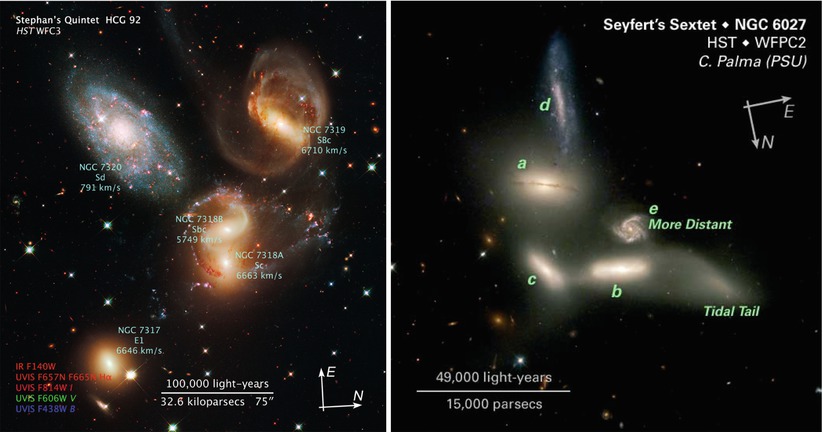
Fig. 6.11
Left
panel: Stephan’s Quintet, also known as Hickson Compact
Group 92, is a very dense accumulation of galaxies with a diameter
of about 80 kpc. The galaxy at the upper left (NGC 7320) is not a
member of the group: its redshift indicates that it has a much
smaller distance from us than the other four galaxies; in fact, it
is close enough to us for HST being able to resolve individual
stars. This galaxy has only ∼ 2 % of the luminosity of the other
galaxies shown, i.e., it is an actively star-forming dwarf galaxy,
as is also seen by its much bluer color compared to the other
galaxies in the field. The remaining three spiral galaxies of the
group show clear signs of interactions—distorted spiral arms and
tidal tails. The strong interaction of the galaxy pair in the
middle of the image gives rise to a strong burst of star formation.
The elliptical galaxy at the bottom left appears to be less
affected by galaxy interactions. The image is a color composite of
optical and near-IR images, as well as a narrow band image at the
Hα wavelength, all taken
with the WFC3 instrument onboard HST. Right panel: Seyfert’s Sextet, an
apparent accumulation of six galaxies located very close together
on the sphere. Only four of the galaxies (a–d) in fact belong to
the group; the spiral galaxy (e) is located at significantly larger
distance. Another object originally classified as a galaxy is no
galaxy but instead a tidal tail that was ejected in tidal
interactions of galaxies in the group. Credit: Left: NASA, ESA, and the Hubble SM4 ERO
Team; Right: NASA, J.
English (U. Manitoba), C. Palma, S. Hunsberger, S. Zonak, J.
Charlton, S. Gallagher (PSU), and L. Frattare (STScI)
Follow-up spectroscopic studies of the HCGs have
verified that 92 of them have at least three galaxies with
conforming redshifts, defined such that the corresponding recession
velocities lie within 1000 km/s of the median velocity of group
members. Of course, the similarity in redshift does not necessarily
imply that these groups form a gravitationally bound and relaxed
system. For instance, the galaxies could be tracers of an overdense
structure which we happen to view from a direction where the
galaxies are projected near each other on the sky. However, more
than 40 % of the galaxies in HCGs show evidence of interactions,
indicating that these galaxies have near neighbors in
three-dimensional space. Furthermore, about three quarters of HCGs
with four or more member galaxies show extended X-ray emission,
most likely coming from intra-group hot gas, providing additional
evidence for the presence of a common gravitational potential well
(see Sect. 6.4). Compared to clusters, the intergalactic
gas in groups has a lower temperature and, possibly, lower
metallicity.
6.2.4 Modern optical cluster catalogs
The subjectivity of selecting overdensities on
images by eye can of course be overcome by using digital (or
digitized) astronomical images and employing algorithms to apply
criteria to the data which define an overdensity, or a cluster,
respectively. This approach solves one of the aforementioned
problems in optical cluster searches. The other problem—namely
projection effects—can be overcome if an additional distance
measure for potential member galaxies can be applied.3 There are two ways how such a
distance indicator can be obtained: one either uses large
spectroscopic catalogs of galaxies, such as the SDSS, or, as will
be discussed next, one can employ the colors of early-type
galaxies.
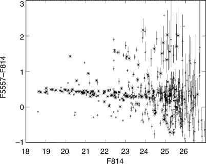
Fig. 6.12
Color-magnitude diagram of the cluster of
galaxies Abell 2390, observed with the HST. Star symbols represent early-type
galaxies, identified by their morphology, while diamonds denote other galaxies in the
field. The red cluster sequence is clearly visible. Note that, due
to projection effects, not all galaxies shown here are indeed
cluster members; some of them are foreground or background
galaxies. Source: M. Gladders & H. Yee 2000, A New Method For Galaxy Cluster Detection. I.
The Algorithm, AJ 120, 2148, p. 2150, Fig. 1. ©AAS.
Reproduced with permission
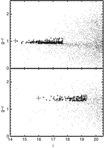
Fig. 6.13
Example of two clusters found by the maxBCG
method. Shown are the color-magnitude relations for galaxies in the
field of Abell 2142 at z = 0. 092 (top) and Abell 1682 at z = 0. 23 (bottom). In both cases, all galaxies
within 2h −1 Mpc
of the BCG are plotted as small
dots. The BCG itself is denoted by a big cross, being the most luminous of
the cluster members, whereas the smaller crosses show galaxies with
L ≥ 0. 4L ∗ whose colors lie within
± 2σ of the red sequence,
which is 0. 05 and 0. 06 for the g − r and r − i, respectively. If they lie closer
that the estimated R
200 from the BCG, they are considered to be cluster
members. We note that the red sequence has almost zero slope in the
color shown here. Although these two clusters were known before,
their rediscovery provides one of the tests of the method. Source:
B.P. Koester et al. 2007, MaxBCG: A Red-Sequence Galaxy Cluster
Finder, ApJ 660, 221, p. 224, Fig. 1. ©AAS. Reproduced
with permission
Color-magnitude
diagram. We mentioned before that a large fraction of
galaxies in clusters are early-type galaxies. Furthermore, we saw
in Sect. 3.6 that early-type galaxies have
rather uniform colors. Indeed, plotting the color of cluster
galaxies versus their magnitude, one finds a very well-defined,
nearly horizontal sequence (Fig. 6.12). This red cluster sequence (RCS) is
populated by the early-type galaxies in the cluster.
The scatter of early-type galaxies around this
sequence is very small, which suggests that all early-type galaxies
in a cluster have nearly the same color, only weakly depending on
luminosity. The small slope seen in Fig. 6.12 is mainly due to the
fact that more massive ellipticals have a somewhat higher
metallicity, rendering the stellar emission slightly redder. Even
more surprising is the fact that the color-magnitude diagrams of
different clusters at the same redshift define a very similar red
cluster sequence: early-type cluster galaxies with the same
redshift and luminosity have virtually the same color. Comparing
the red sequences of clusters at different redshifts, one finds
that the sequence of cluster galaxies is redder the higher the
redshift is. This effect is caused by the redshift of the galaxies,
which shift their spectral energy distribution towards longer
wavelengths. Hence, by keeping the observed filter bands constant,
the colors change as a function of redshift. In fact, the red
cluster sequence is so precisely characterized that, from the
color-magnitude diagram of a cluster alone, its redshift can be
estimated with very high accuracy, provided the photometric
calibration is sufficiently good. Furthermore, the accuracy of this
estimated redshift strongly depends on the choice of the filters
between which the color is measured. Since the most prominent
spectral feature of early-type galaxies is the 4000 Å-break, the
redshift is estimated best if this rest-frame wavelength,
redshifted to 4000 (1 + z) Å, is well covered by the
photometric bands employed.
This well-defined red cluster sequence is of
crucial importance for our understanding of the evolution of
galaxies. We know from Sect. 3.5 that the composition of a
stellar population depends on the mass spectrum at its birth (the
initial mass function, IMF) and on its age: the older a population
is, the redder it becomes. The fact that cluster galaxies at the
same redshift all have roughly the same color indicates that their
stellar populations have very similar ages. However, the only age
that is singled out is the age of the Universe itself. In fact, the
color of cluster galaxies is compatible with their stellar
populations being roughly the same age as the Universe at that
particular redshift. This also provides an explanation for why the
red cluster sequence is shifted towards intrinsically bluer colors at higher
redshifts—there, the age of the Universe was smaller, and thus the
stellar population was younger. This effect is of particular
importance at high redshifts.
The RCS
Survey. The cluster red sequence method was used in several
multi-band imaging surveys for the detection of clusters. In fact,
one of the large imaging surveys carried out with the CFHT was the
RCS survey, with its main purpose to detect clusters out to large
redshifts. It covered 100 deg2 in two filters, and
yielded more than 1000 cluster and group candidates, out to
redshifts larger than unity. As a follow-up, the RCS II survey
covers 900 deg2 in three filters, and aims at detecting
some 104 clusters out to z ∼ 1.
The maxBCG
catalog. The large sky coverage of the SDSS, and the very
homogeneous photometry of the five-band imaging data, makes this
survey a prime resource for optical cluster finders. Whereas the
SDSS is rather shallow, compared to the RCS surveys, and thus
cannot find clusters at high redshifts, it enables the most
complete cluster searches in the more local Universe. Therefore,
several cluster catalogs have been constructed from the SDSS, one
of which we want to briefly describe here.
This maxBCG cluster catalog is based on a search
algorithm which makes use of three properties of massive clusters.
The first is the already mentioned red cluster sequence, i.e., the
homogeneous (and redshift dependent) color of early-type galaxies
in clusters. Second, most massive clusters are found to have a
dominant central galaxy, the brightest cluster galaxy (BCG), whose
luminosity can be several times larger than the second brightest
cluster member. The third property relates to the radial density
profile of galaxies, which, in a first approximation, decreases
roughly as 1∕θ from the
center to the outside.
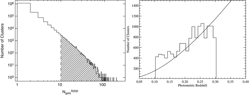
Fig. 6.14
Left: Histogram of the number of
clusters found by the maxBCG method, as a function of cluster
richness N
g,200. The maxBCG catalog consists of 13 823 clusters
with N
g,200 ≥ 10, shown as hatched region in the histogram.
The right panel shows the
distribution of estimated redshifts, whereas the solid curve is the expected redshift
distribution for a volume-limited survey with the sky area of the
SDSS at a given mean number density of  . Source:
B.P. Koester et al. 2007, A
MaxBCG Catalog of 13,823 Galaxy Clusters from the Sloan Digital Sky
Survey, ApJ 660, 239, p. 243, 244, Figs. 3, 4.
©AAS. Reproduced with permission
. Source:
B.P. Koester et al. 2007, A
MaxBCG Catalog of 13,823 Galaxy Clusters from the Sloan Digital Sky
Survey, ApJ 660, 239, p. 243, 244, Figs. 3, 4.
©AAS. Reproduced with permission
. Source:
B.P. Koester et al. 2007, A
MaxBCG Catalog of 13,823 Galaxy Clusters from the Sloan Digital Sky
Survey, ApJ 660, 239, p. 243, 244, Figs. 3, 4.
©AAS. Reproduced with permissionThus, the algorithm searches for overdensities of
galaxies with similar color, corresponding to the color of the red
sequence within a specified redshift interval, where the brightest
of the galaxies is located near the center of the overdensity, and
where the radial decline of the galaxy number density is compatible
with a 1∕θ-law. More
specifically, the maxBCG method searches for concentrations of
luminous red galaxies in the redshift interval 0. 1 ≲ z ≲ 0. 3, whose colors agree to within
± 2σ of the width of the
red sequence in color and with the brightest of these galaxies near
the center (Fig. 6.13). The choice of this redshift interval is
motivated by the fact that the g − r color of red galaxies is a simple
function of redshift, as the strong 4000 Å-break of early-type
galaxies moves through the g-filter in this redshift interval. The
color of the overdense population yields an indication of the
redshift, which then allows one to obtain the galaxy luminosity
from the observed flux. Only red galaxies more luminous than
0. 4L ∗ are
taken into account. Given the depth of the SDSS, a red galaxy with
L ≥ 0. 4L ∗ at z = 0. 3 can be detected—hence, this
provides a volume-limited survey for such galaxies. Furthermore,
the redshift estimate is used to obtain the physical projected
radius R from the observed
angular separation.
To characterize the cluster candidate, the number
of red sequence galaxies with L ≥ 0. 4L ∗ within 1h −1 Mpc of the BCG
candidate, N g,
is calculated. For reasons that will become clear when we discuss
the formation of dark matter halos in Sect. 7.5.1 (see also
Problem 6.1), one defines the ‘extent’ of a cluster to
be the radius inside of which the mean density is 200 times larger
than the critical density of the Universe at this redshift. This
radius is denoted by r
200, and the mass of the cluster within r 200 is then denoted as
 ,
often also called the virial mass of the cluster. From earlier
cluster studies, it was found that there is a close relation
between r 200
(or M 200) and
the number of galaxies within 1h −1 Mpc, roughly following
r
200 ∝ N
g. With this estimate of the virial radius, the number
of red sequence members within projected radius R = r 200 is measured and
denoted by N
g,200, which is then called the richness of the
cluster.
,
often also called the virial mass of the cluster. From earlier
cluster studies, it was found that there is a close relation
between r 200
(or M 200) and
the number of galaxies within 1h −1 Mpc, roughly following
r
200 ∝ N
g. With this estimate of the virial radius, the number
of red sequence members within projected radius R = r 200 is measured and
denoted by N
g,200, which is then called the richness of the
cluster.These criteria have yielded a catalog of 13 823
clusters with N
g,200 ≥ 10 in the 7500 deg2 of the SDSS.
Their distribution in richness and redshift is shown in
Fig. 6.14.
This maxBCG catalog is one of the largest cluster catalogs
available up to now and has been widely used.
The quality of the catalog can be assessed in a
number of ways. Since the SDSS also has a large spectroscopic
component, the spectroscopic redshifts for more than 5000 of the
BCGs are known; they can be compared to the redshift estimated from
the color of the red-sequence cluster members. The difference
between the two redshifts has a very narrow distribution with a
width of σ
z ∼ 0. 01—that
is, the estimated cluster redshifts are very accurate.
A good catalog should be pure and complete. As
mentioned before, purity measures the fraction of objects included
in the catalog which are not real clusters, whereas completeness
quantifies the number of real clusters which were missed by the
selection algorithm. These two quantities can be estimated from
simulations, in which mock cluster catalogs are generated and
analyzed with the same detection algorithm as the real data. Based
on such simulations, one concludes that the maxBCG catalog
is ∼ 90 % pure and ∼ 85 % complete, for clusters with masses
 , corresponding to
N
g,200 ≈ 10.
, corresponding to
N
g,200 ≈ 10.
, corresponding to
N
g,200 ≈ 10.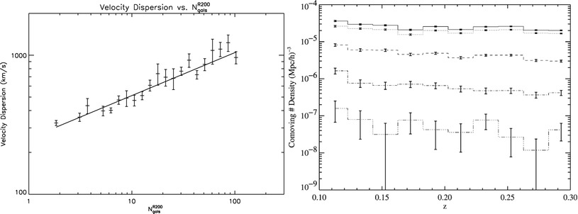
Fig. 6.15
Left: The velocity dispersion of maxBCG
clusters, as a function of richness N g,200. Note that the
figure extends to richness as small as N g,200 = 2. At the
threshold of the cluster catalog, N g,200 = 10, the
characteristic velocity dispersion is ∼ 500 km∕s. Right: The comoving number density of
clusters in the maxBCG catalog, as a function of redshift, for four
different redshift bins (from top
to bottom: 10 ≤ N
g,200 < 20, 20 ≤ N g,200 < 43,
43 ≤ N
g,200 < 91, 91 ≤ N g,200 < 189). Source:
B.P. Koester et al. 2007, A
MaxBCG Catalog of 13,823 Galaxy Clusters from the Sloan Digital Sky
Survey, ApJ 660, 239, p. 251, Figs. 12, 13. ©AAS.
Reproduced with permission
The available spectroscopy of the SDSS can also
be used to determine the velocity dispersion σ v for many of the clusters. The
left panel of Fig. 6.15 shows a strong correlation between
σ v and richness, well fit by a
power law of the form
 This strong correlation also shows that cluster richness is a good
indicator of cluster mass, since σ v is expected to be tightly
related to the mass, according to the virial theorem; we will
return to this aspect soon. The comoving number density of clusters
as a function of redshift is shown in the right panel of
Fig. 6.15,
for different richness bins. The comoving space density is roughly
constant for all bins except for the richest, which suggests that
the maxBCG catalog does not suffer from serious redshift-dependent
incompleteness. The slight decline with increasing redshift in the
richest bin is actually expected from structure formation in the
Universe, as we will discuss in Sect. 7.5.2.
This strong correlation also shows that cluster richness is a good
indicator of cluster mass, since σ v is expected to be tightly
related to the mass, according to the virial theorem; we will
return to this aspect soon. The comoving number density of clusters
as a function of redshift is shown in the right panel of
Fig. 6.15,
for different richness bins. The comoving space density is roughly
constant for all bins except for the richest, which suggests that
the maxBCG catalog does not suffer from serious redshift-dependent
incompleteness. The slight decline with increasing redshift in the
richest bin is actually expected from structure formation in the
Universe, as we will discuss in Sect. 7.5.2.
(6.7)
For candidates with N g,200 < 10, i.e., mass
below  , the purity and
completeness decrease; hence, whereas a large fraction of these
candidates are probably clusters or groups at lower mass,
projection effects will play an increasingly important role for
decreasing richness. To reliably find groups, the selection
criteria need to be sharpened, which can be done using
spectroscopic redshifts. With those, one can search for galaxy
overdensities on the sky which have the same redshifts within a few
times the expected velocity dispersion in groups, i.e., the same
radial velocity within ∼ 1000 km∕s. This provides a much stricter
redshift constraint than is possible with the red sequence method
and thus substantially reduces projection effects. Such group
catalogs were constructed from the Two-degree field Galaxy Redshift
Survey (see Sect. 8.1.2) and the SDSS as well. The
velocity dispersion in groups is significantly smaller than that in
clusters; typical values for groups with only a few members are
σ v ∼ 300 km∕s (see
Fig. 6.15).
, the purity and
completeness decrease; hence, whereas a large fraction of these
candidates are probably clusters or groups at lower mass,
projection effects will play an increasingly important role for
decreasing richness. To reliably find groups, the selection
criteria need to be sharpened, which can be done using
spectroscopic redshifts. With those, one can search for galaxy
overdensities on the sky which have the same redshifts within a few
times the expected velocity dispersion in groups, i.e., the same
radial velocity within ∼ 1000 km∕s. This provides a much stricter
redshift constraint than is possible with the red sequence method
and thus substantially reduces projection effects. Such group
catalogs were constructed from the Two-degree field Galaxy Redshift
Survey (see Sect. 8.1.2) and the SDSS as well. The
velocity dispersion in groups is significantly smaller than that in
clusters; typical values for groups with only a few members are
σ v ∼ 300 km∕s (see
Fig. 6.15).6.3 Light distribution and cluster dynamics
6.3.1 Spatial distribution of galaxies
Most regular clusters show a centrally condensed
number density distribution of cluster galaxies, i.e., the galaxy
density increases strongly towards the center. If the cluster is
not very elongated, this density distribution can be assumed, to a
first approximation, as being spherically symmetric. Only the
projected density distribution N(R) is observable. This is related to
the three-dimensional number density n(r) through
 where in the second step a simple transformation of the integration
variable from the line-of-sight coordinate r 3 to the three-dimensional
radius
where in the second step a simple transformation of the integration
variable from the line-of-sight coordinate r 3 to the three-dimensional
radius  was made.
(6.8)
was made.Of course, no function N(R) can be observed, but only points
(the positions of the galaxies) that are distributed in a certain
way. If the number density of galaxies is sufficiently large,
N(R) is obtained by smoothing the point
distribution. Alternatively, one considers parametrized forms of
N(R) and fits the parameters to the
observed galaxy positions. In most cases, the second approach is
taken because its results are more robust. A parametrized
distribution needs to contain at least five parameters to be able
to describe at least the basic characteristics of a cluster. Two of
these parameters describe the position of the cluster center on the
sky. One parameter is used to describe the amplitude of the
density, for which, e.g., the central density N 0 = N(0) may be used. A fourth parameter is
a characteristic scale of a cluster, often taken to be the core
radius r c,
defined such that at R = r c, the projected density
has decreased to half the central value,  . Finally, one parameter
is needed to describe ‘where the cluster ends’; the Abell radius is
a first approximation for such a parameter.4
. Finally, one parameter
is needed to describe ‘where the cluster ends’; the Abell radius is
a first approximation for such a parameter.4
. Finally, one parameter
is needed to describe ‘where the cluster ends’; the Abell radius is
a first approximation for such a parameter.4Parametrized cluster models can be divided into
those which are physically motivated, and those which are of a
purely mathematical nature. One example for the latter is the
family of Sérsic profiles which is not derived from dynamical
models. Next, we will consider a class of distributions that are
based on a dynamical model.
Isothermal
distributions. These models are based on the assumption that
the velocity distribution of the massive particles (this may be
both galaxies in the cluster or dark matter particles) of a cluster
is locally described by a Maxwell distribution, i.e., they are
‘thermalized’. As shown from spectroscopic analyses of the
distribution of the radial velocities of cluster galaxies, this is
not a bad assumption. Assuming, in addition, that the mass profile
of the cluster follows that of the galaxies (or vice versa), and
that the temperature (or equivalently the velocity dispersion) of
the distribution does not depend on the radius, so that one has an
isothermal distribution of galaxies, then one obtains a
one-parameter set of models, the so-called isothermal spheres. These can be
described physically as follows.
In dynamical equilibrium, the pressure gradient
must be equal to the gravitational acceleration, so that
 where ρ(r) denotes the density of the
distribution, e.g., the density of galaxies. By
where ρ(r) denotes the density of the
distribution, e.g., the density of galaxies. By  ,
this mass density is related to the number density n(r), where
,
this mass density is related to the number density n(r), where  is the average
particle mass.
is the average
particle mass.  is the mass of the cluster enclosed within a radius r. By differentiation
of (6.9),
we obtain
is the mass of the cluster enclosed within a radius r. By differentiation
of (6.9),
we obtain
 The relation between pressure and density is P = nk B T. On the other hand, the temperature
is related to the velocity dispersion of the particles,
The relation between pressure and density is P = nk B T. On the other hand, the temperature
is related to the velocity dispersion of the particles,
 where
where  is the mean
squared velocity, i.e., the velocity dispersion, provided the
average velocity vector is set to zero. The latter assumption means
that the cluster does not rotate, or contract or expand. If
T (or
is the mean
squared velocity, i.e., the velocity dispersion, provided the
average velocity vector is set to zero. The latter assumption means
that the cluster does not rotate, or contract or expand. If
T (or  ) is independent
of r, then
) is independent
of r, then
 where σ v 2 is the
one-dimensional velocity dispersion, e.g., the velocity dispersion
along the line-of-sight, which can be measured from the redshifts
of the cluster galaxies. If the velocity distribution corresponds
to an isotropic (Maxwell) distribution, the one-dimensional
velocity dispersion is exactly 1/3 times the three-dimensional
velocity dispersion, because of
where σ v 2 is the
one-dimensional velocity dispersion, e.g., the velocity dispersion
along the line-of-sight, which can be measured from the redshifts
of the cluster galaxies. If the velocity distribution corresponds
to an isotropic (Maxwell) distribution, the one-dimensional
velocity dispersion is exactly 1/3 times the three-dimensional
velocity dispersion, because of  ,
or
,
or
 With (6.10), it then follows that

(6.9)
,
this mass density is related to the number density n(r), where is the average
particle mass.
is the mass of the cluster enclosed within a radius r. By differentiation
of (6.9),
we obtain
(6.10)
(6.11)
is the mean
squared velocity, i.e., the velocity dispersion, provided the
average velocity vector is set to zero. The latter assumption means
that the cluster does not rotate, or contract or expand. If
T (or ) is independent
of r, then
(6.12)
,
or
(6.13)
(6.14)
Singular
isothermal sphere. For general boundary conditions, the
differential equation (6.14) for ρ(r) cannot be solved analytically.
However, one particular analytical solution of the differential
equation exists: By substitution, we can easily show that
 solves (6.14). This density distribution is called
singular isothermal sphere;
we have encountered it before, in the discussion of gravitational
lens models in Sect. 3.11.2. This distribution has a
diverging density as r → 0
and an infinite total mass M(r) ∝ r. It is remarkable that this density
distribution, ρ ∝ r −2, is just what is needed
to explain the flat rotation curves of galaxies at large
radii.
solves (6.14). This density distribution is called
singular isothermal sphere;
we have encountered it before, in the discussion of gravitational
lens models in Sect. 3.11.2. This distribution has a
diverging density as r → 0
and an infinite total mass M(r) ∝ r. It is remarkable that this density
distribution, ρ ∝ r −2, is just what is needed
to explain the flat rotation curves of galaxies at large
radii.
(6.15)
The divergence of the density towards the center
may not appear reasonable, and thus one might search solutions
of (6.14) with the more physical boundary
conditions ρ(0) = ρ 0, the central density,
and  , for
the density profile to be flat at the center. Numerical solutions
of (6.14) with these boundary conditions (thus,
with a flat core) reveal that the central density and the core
radius are related to each other by
, for
the density profile to be flat at the center. Numerical solutions
of (6.14) with these boundary conditions (thus,
with a flat core) reveal that the central density and the core
radius are related to each other by
 Hence, these physical solutions of (6.14) avoid the infinite
density of the singular isothermal sphere. However, these solutions
also decrease outwards with ρ ∝ r −2, so they have a
diverging mass as well. The origin of this mass divergence is
easily understood because these isothermal distributions are based
on the assumption that the velocity distribution is isothermal,
thus Maxwellian with a spatially constant temperature. A Maxwell
distribution has wings, hence it (formally) contains particles with
arbitrarily high velocities. Since the distribution is assumed
stationary, such particles must not escape, so their velocity must
be lower than the escape velocity from the gravitational well of
the cluster. But for a Maxwell distribution this is only achievable
for an infinite total mass.
Hence, these physical solutions of (6.14) avoid the infinite
density of the singular isothermal sphere. However, these solutions
also decrease outwards with ρ ∝ r −2, so they have a
diverging mass as well. The origin of this mass divergence is
easily understood because these isothermal distributions are based
on the assumption that the velocity distribution is isothermal,
thus Maxwellian with a spatially constant temperature. A Maxwell
distribution has wings, hence it (formally) contains particles with
arbitrarily high velocities. Since the distribution is assumed
stationary, such particles must not escape, so their velocity must
be lower than the escape velocity from the gravitational well of
the cluster. But for a Maxwell distribution this is only achievable
for an infinite total mass.
, for
the density profile to be flat at the center. Numerical solutions
of (6.14) with these boundary conditions (thus,
with a flat core) reveal that the central density and the core
radius are related to each other by
(6.16)
King
models. To remove the problem of the diverging total mass,
self-gravitating dynamical models with an upper cut-off in the
velocity distribution of their constituent particles are
introduced. These are called King
models and cannot be expressed analytically. However, an
analytical approximation exists for the central region of these
mass profiles,
![$$\displaystyle\begin{array}{rcl} \fbox{$\rho (r) =\rho _{0}\left [1 + \left ( \frac{r} {r_{\mathrm{c}}}\right )^{2}\right ]^{-3/2}$}\;.& &{}\end{array}$$](A129044_2_En_6_Chapter_Equ17.gif) Using (6.8), we obtain from this the projected surface
mass density
Using (6.8), we obtain from this the projected surface
mass density
![$$\displaystyle\begin{array}{rcl} \fbox{$\varSigma (R) =\varSigma _{0}\left [1 + \left ( \frac{R} {r_{\mathrm{c}}}\right )^{2}\right ]^{-1} \mathrm{with} \varSigma _{ 0} = 2\rho _{0}r_{\mathrm{c}}$}\;.& &{}\end{array}$$](A129044_2_En_6_Chapter_Equ18.gif) The analytical fit (6.17) of the King profile also has a diverging
total mass, but this divergence is ‘only’ logarithmic.
The analytical fit (6.17) of the King profile also has a diverging
total mass, but this divergence is ‘only’ logarithmic.
(6.17)
(6.18)
These analytical models for the density
distribution of galaxies in clusters are only approximations, of
course, because the galaxy distribution in clusters is often
heavily structured. Furthermore, these dynamical models are
applicable to a galaxy distribution only if the galaxy number
density follows the matter density. However, one finds that the
distribution of galaxies in a cluster often depends on the galaxy
type. The fraction of early-type galaxies (Es and S0s) is often
largest near the center. Therefore, one should consider the
possibility that the distribution of galaxies in a cluster may be
different from that of the total matter. A typical value for the
core radius is about r
c ∼ 0. 25h
−1 Mpc.
6.3.2 Dynamical mass of clusters
The above argument relates the velocity
distribution of cluster galaxies to the mass profile of the
cluster, and from this we obtain physical models for the density
distribution. This implies the possibility of deriving the mass, or
the mass profile, respectively, of a cluster from the observed
velocities of cluster galaxies. We will briefly present this method
of mass determination here. For this, we consider the dynamical
time-scale of clusters, defined as the time a typical galaxy needs
to traverse the cluster once,
 where a (one-dimensional) velocity dispersion σ v ∼ 1000 km∕s was assumed. The
dynamical time-scale is shorter than the age of the Universe. One
therefore concludes that clusters of galaxies are gravitationally
bound systems. If this were not the case they would dissolve on a
timescale t
cross. Since t
cross ≪ t
0 one assumes a virial
equilibrium, hence that the virial theorem applies, so that
in a time-average sense,
where a (one-dimensional) velocity dispersion σ v ∼ 1000 km∕s was assumed. The
dynamical time-scale is shorter than the age of the Universe. One
therefore concludes that clusters of galaxies are gravitationally
bound systems. If this were not the case they would dissolve on a
timescale t
cross. Since t
cross ≪ t
0 one assumes a virial
equilibrium, hence that the virial theorem applies, so that
in a time-average sense,
 where
where
 are the kinetic and the potential energy of the cluster galaxies,
m i is the mass of the i-th galaxy, v i is the absolute value of its
velocity, and r
ij is the
spatial separation between the i-th and the j-th galaxy. The factor 1∕2 in the
definition of E
pot occurs since each pair of galaxies occurs twice in
the sum.
are the kinetic and the potential energy of the cluster galaxies,
m i is the mass of the i-th galaxy, v i is the absolute value of its
velocity, and r
ij is the
spatial separation between the i-th and the j-th galaxy. The factor 1∕2 in the
definition of E
pot occurs since each pair of galaxies occurs twice in
the sum.
(6.19)
(6.20)
(6.21)
In writing (6.21) we have assumed
that the total mass of the cluster is the sum of all its member
galaxies,
 This assumption is not valid, since, as we will find below, most of
the cluster mass is not contained in galaxies. However, if we
assume that the total mass is distributed in the same way as the
galaxies are, we can associate to each galaxy a ‘representative’
mass, so that the superposition of all these representative masses
yields the total mass distribution of the cluster. The mass
m i used in the foregoing equations
and below is meant to be this representative mass.
This assumption is not valid, since, as we will find below, most of
the cluster mass is not contained in galaxies. However, if we
assume that the total mass is distributed in the same way as the
galaxies are, we can associate to each galaxy a ‘representative’
mass, so that the superposition of all these representative masses
yields the total mass distribution of the cluster. The mass
m i used in the foregoing equations
and below is meant to be this representative mass.
(6.22)
We further define the velocity dispersion,
weighted by mass,
 and the gravitational radius,
 With this, we obtain
 for the kinetic and potential energy. Applying the virial
theorem (6.20) yields the mass estimate
for the kinetic and potential energy. Applying the virial
theorem (6.20) yields the mass estimate

(6.23)
(6.24)
(6.25)
(6.26)
Transition to
projected quantities. The above derivation uses the
three-dimensional separations r i of the galaxies from the
cluster center, which are, however, not observable. To be able to
apply these equations to observations, they need to be transformed
to projected separations. If the galaxy positions and the
directions of their velocity vectors are uncorrelated, as it is the
case, e.g., for an isotropic velocity distribution, then
 where R ij denotes the projected
separation between the galaxies i and j. The parameters σ v and R G are direct observables;
thus, the total mass of the cluster can be determined. One obtains
where R ij denotes the projected
separation between the galaxies i and j. The parameters σ v and R G are direct observables;
thus, the total mass of the cluster can be determined. One obtains
 We explicitly point out that this mass estimate no longer depends
on the masses m
i of the
individual galaxies—rather the galaxies are now test particles in
the gravitational potential. With σ v ∼ 1000 km∕s and R G ∼ 1 Mpc as typical
values for rich clusters of galaxies, one obtains a characteristic
mass of
We explicitly point out that this mass estimate no longer depends
on the masses m
i of the
individual galaxies—rather the galaxies are now test particles in
the gravitational potential. With σ v ∼ 1000 km∕s and R G ∼ 1 Mpc as typical
values for rich clusters of galaxies, one obtains a characteristic
mass of  for rich clusters.
(6.27)
(6.28)
for rich clusters.The ‘missing mass’
problem in clusters of galaxies. With the mass M and the number N of galaxies, one can now derive a
characteristic mass  for the luminous galaxies. This mass is
found to be very high,
for the luminous galaxies. This mass is
found to be very high,  . Alternatively,
M can be compared with the
total optical luminosity of the cluster galaxies, L
tot ∼ 1012-
. Alternatively,
M can be compared with the
total optical luminosity of the cluster galaxies, L
tot ∼ 1012- , and hence the mass-to-light
ratio can be calculated; typically
, and hence the mass-to-light
ratio can be calculated; typically
 This value exceeds the M∕L-ratio of early-type galaxies by at
least a factor of 10. Realizing this discrepancy, Fritz Zwicky
concluded as early as 1933, from an analysis of the Coma cluster,
that clusters of galaxies must contain considerably more mass than
is visible in galaxies—the dawn of the missing mass problem. As we will see
further below, this discrepancy between the observed luminosity and
estimated mass has by now been firmly established, since other
methods for the mass determination of clusters also yield
comparable values and indicate that a major fraction of the mass in
galaxy clusters consists of (non-baryonic) dark matter.
The stars visible in galaxies
contribute less than about 5 % to the total mass in clusters of
galaxies.
This value exceeds the M∕L-ratio of early-type galaxies by at
least a factor of 10. Realizing this discrepancy, Fritz Zwicky
concluded as early as 1933, from an analysis of the Coma cluster,
that clusters of galaxies must contain considerably more mass than
is visible in galaxies—the dawn of the missing mass problem. As we will see
further below, this discrepancy between the observed luminosity and
estimated mass has by now been firmly established, since other
methods for the mass determination of clusters also yield
comparable values and indicate that a major fraction of the mass in
galaxy clusters consists of (non-baryonic) dark matter.
The stars visible in galaxies
contribute less than about 5 % to the total mass in clusters of
galaxies.
for the luminous galaxies. This mass is
found to be very high, . Alternatively,
M can be compared with the
total optical luminosity of the cluster galaxies, L
tot ∼ 1012-, and hence the mass-to-light
ratio can be calculated; typically
(6.29)
Fig. 6.16
The principle of dynamical friction. The
gravitational field of a massive particle (here indicated by the
large symbol) accelerates
the surrounding matter towards its track. Through this, an
overdensity establishes on the backward side of its orbit, the
gravitational force of which decelerates the particle
6.3.3 Additional remarks on cluster dynamics
Given the above line of argument, the question of
course arises as to whether the application of the virial theorem
is still justified if the main fraction of mass is not contained in
galaxies. The derivation remains valid in this form as long as the
spatial distribution of galaxies follows the total mass
distribution. The dynamical mass determination can be affected by
an anisotropic velocity distribution of the cluster galaxies and by
the possibly non-spherical cluster mass distribution. In both
cases, projection effects, which are dealt with relatively easily
in the spherically-symmetric case, obviously become more
complicated. This is also one of the reasons for the necessity to
consider alternative methods of mass determination.
Two-body collisions of galaxies in clusters are
of no importance dynamically, as is easily seen from the
corresponding relaxation time-scale (3.3),
 which is much larger than the age of the Universe. The motion of
galaxies is therefore governed by the collective gravitational
potential of the cluster. The velocity dispersion is approximately
the same for the different types of galaxies, and also only a weak
tendency exists for a dependence of σ v on galaxy luminosity,
restricted to the brightest ones (see below in Sect. 6.7.2). From this, we
conclude that the galaxies in a cluster are not “thermalized”
because this would mean that they all have the same mean kinetic
energy, implying
which is much larger than the age of the Universe. The motion of
galaxies is therefore governed by the collective gravitational
potential of the cluster. The velocity dispersion is approximately
the same for the different types of galaxies, and also only a weak
tendency exists for a dependence of σ v on galaxy luminosity,
restricted to the brightest ones (see below in Sect. 6.7.2). From this, we
conclude that the galaxies in a cluster are not “thermalized”
because this would mean that they all have the same mean kinetic
energy, implying  . Furthermore, the
independence of σ
v of
L reconfirms that
collisions of galaxies with each other are not dynamically
relevant; rather, the velocity distribution of galaxies is defined
by collective processes during cluster formation.
. Furthermore, the
independence of σ
v of
L reconfirms that
collisions of galaxies with each other are not dynamically
relevant; rather, the velocity distribution of galaxies is defined
by collective processes during cluster formation.
. Furthermore, the
independence of σ
v of
L reconfirms that
collisions of galaxies with each other are not dynamically
relevant; rather, the velocity distribution of galaxies is defined
by collective processes during cluster formation.Violent
relaxation. One of the most important of the aforementioned
processes is known as violent
relaxation. This process very quickly establishes a virial
equilibrium in the course of the gravitational collapse of a mass
concentration. The reason for it are the small-scale density
inhomogeneities within the collapsing matter distribution which
generate, via Poisson’s equation, corresponding fluctuations in the
gravitational field. These then scatter the infalling particles
and, by this, the density inhomogeneities are further amplified.
The fluctuations of the gravitational field act on the matter like
scattering centers. In addition, these field fluctuations change
over time, yielding an effective exchange of energy between the
particles. In a statistical average, all galaxies obtain the same
velocity distribution by this process. As confirmed by numerical
simulations, this process takes place on a time-scale of
t cross, i.e.,
roughly as quickly as the collapse itself.
Dynamical
friction. Another important process for the dynamics of
galaxies in a cluster is dynamical
friction. The simplest picture of dynamical friction is
obtained by considering the following. If a massive particle of
mass m moves through a
statistically homogeneous distribution of massive particles, the
gravitational force on this particle vanishes due to homogeneity.
But since the particle itself has a mass, it will attract other
massive particles and thus cause the distribution to become
inhomogeneous. As the particle moves, the surrounding ‘background’
particles will react to its gravitational field and slowly start
moving towards the direction of the particle trajectory. Due to the
inertia of matter, the resulting density inhomogeneity will be such
that an overdensity of mass will be established along the track of
the particle, where the density will be higher on the side opposite
to the direction of motion (thus, behind the particle) than in the
forward direction (see Fig. 6.16). By this process, a gravitational field
will form that causes an acceleration of the particle against the
direction of motion, so that the particle will be slowed down.
Because this ‘polarization’ of the medium is caused by the gravity
of the particle, which is proportional to its mass, the
deceleration will also be proportional to m. Furthermore, a fast-moving particle
will cause less polarization in the medium than a slowly moving one
because each mass element in the medium is experiencing the
gravitational attraction of the particle for a shorter time, thus
the medium becomes less polarized. In addition, the particle is on
average farther away from the density accumulation on its backward
track, and thus will experience a smaller acceleration if it is
faster. Combining these arguments, one obtains for the dependence
of this dynamical friction
 where ρ is the mass density
in the medium. Applied to clusters of galaxies, this means that the
most massive galaxies will experience the strongest dynamical
friction, so that they are subject to a significant deceleration
through which they move deeper into the potential well. The most
massive cluster galaxies should therefore be concentrated around
the cluster center, so that a spatial separation of galaxy
populations with respect to their masses occurs (mass segregation)
. If dynamical friction acts over a sufficiently long time, the
massive cluster galaxies in the center may merge into a single one.
This is one possible explanation for the formation of cD galaxies.
Furthermore, as the most massive (and thus presumably also the most
luminous) galaxies are affected strongest by dynamical friction,
and are thus the prime candidates for merging with the central
galaxy, this may explain the observed gap of ∼ 2 mag between the
brightest and second brightest cluster galaxy.
where ρ is the mass density
in the medium. Applied to clusters of galaxies, this means that the
most massive galaxies will experience the strongest dynamical
friction, so that they are subject to a significant deceleration
through which they move deeper into the potential well. The most
massive cluster galaxies should therefore be concentrated around
the cluster center, so that a spatial separation of galaxy
populations with respect to their masses occurs (mass segregation)
. If dynamical friction acts over a sufficiently long time, the
massive cluster galaxies in the center may merge into a single one.
This is one possible explanation for the formation of cD galaxies.
Furthermore, as the most massive (and thus presumably also the most
luminous) galaxies are affected strongest by dynamical friction,
and are thus the prime candidates for merging with the central
galaxy, this may explain the observed gap of ∼ 2 mag between the
brightest and second brightest cluster galaxy.
(6.30)
Dynamical friction also plays an important role
in other dynamical processes in astrophysics. For example, the
Magellanic Clouds experience dynamical friction on their orbit
around the Milky Way and thereby lose kinetic energy. Consequently,
their orbit will become smaller over the course of time and, in a
distant future, these two satellite galaxies will merge with our
Galaxy. In fact, dynamical friction is of vital importance in
galaxy merger processes which occur in the evolution of the galaxy
population, a subject we will return to in Chap. 10.
Compact groups have a lifetime which is much
shorter than the age of the Universe. The dynamical time-scale is
 ,
thus small compared to
,
thus small compared to  . By dynamical friction,
galaxies in groups lose kinetic (orbital) energy and move closer to
the dynamical center where interactions and mergers with other
group galaxies take place, as also seen by the high fraction of
member galaxies with morphological signs of interactions. Since the
lifetime of compact groups is shorter than the age of the Universe,
they must have formed not too long ago. If we do not happen to live
in a special epoch of cosmic history, such groups must therefore
still be forming today. From dynamical studies, one estimates
that—as in clusters—the total mass of groups is significantly
larger than the sum of the mass visible in galaxies; a typical
mass-to-light ratio is M∕L ∼ 50h (in Solar units), which is comparable
to that of the Local Group.
. By dynamical friction,
galaxies in groups lose kinetic (orbital) energy and move closer to
the dynamical center where interactions and mergers with other
group galaxies take place, as also seen by the high fraction of
member galaxies with morphological signs of interactions. Since the
lifetime of compact groups is shorter than the age of the Universe,
they must have formed not too long ago. If we do not happen to live
in a special epoch of cosmic history, such groups must therefore
still be forming today. From dynamical studies, one estimates
that—as in clusters—the total mass of groups is significantly
larger than the sum of the mass visible in galaxies; a typical
mass-to-light ratio is M∕L ∼ 50h (in Solar units), which is comparable
to that of the Local Group.
,
thus small compared to . By dynamical friction,
galaxies in groups lose kinetic (orbital) energy and move closer to
the dynamical center where interactions and mergers with other
group galaxies take place, as also seen by the high fraction of
member galaxies with morphological signs of interactions. Since the
lifetime of compact groups is shorter than the age of the Universe,
they must have formed not too long ago. If we do not happen to live
in a special epoch of cosmic history, such groups must therefore
still be forming today. From dynamical studies, one estimates
that—as in clusters—the total mass of groups is significantly
larger than the sum of the mass visible in galaxies; a typical
mass-to-light ratio is M∕L ∼ 50h (in Solar units), which is comparable
to that of the Local Group.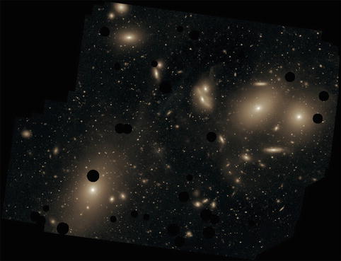
Fig. 6.17
This image shows the central part of the
Virgo cluster, with its central galaxy M87 located in the
lower left corner. The size
of the image is about 1.5∘; it shows the diffuse light
in the cluster between the cluster galaxies. Dark spots indicate regions that were
masked, e.g. because of bright foreground stars. The brightest
parts before saturation have a surface brightness of μ V
∼ 26. 5 mag∕arcsec2, the faintest visible features have
μ V
∼ 28. 5 mag∕arcsec2. Credit: Chris Mihos (Case Western
Reserve University)/European Southern Observatory
6.3.4 Intergalactic stars in clusters of galaxies
The space between the galaxies in a cluster is
filled with hot gas, as visible from X-ray observations. Besides
this hot gas there are also stars in between the galaxies. This
intracluster light (ICL) is
the most recently discovered component in clusters. The detection
of such an intergalactic stellar population comes as a surprise at
first sight, because our understanding of star formation implies
that they can only form in the dense centers of molecular clouds.
Hence, one expects that stars cannot form in intergalactic space.
This is not necessarily implied by the presence of intergalactic
stars, however, since they can also be stripped from galaxies in
the course of gravitational interactions between galaxies in the
cluster, or the stripping of stars from the outer parts of galaxies
in the tidal gravitational field (in the central region) of the
cluster, and so form an intergalactic population. The fate of these
stars is thus somewhat similar to that of the interstellar medium,
which is metal-enriched by the processes of stellar evolution in
galaxies before it is removed from these galaxies and becomes part
of the intergalactic medium in clusters; otherwise, the substantial
metallicity of the ICM could not be explained.5 This interpretation is strengthened
by the fact that a diffuse optical light component is also seen in
(compact) galaxy groups where the strength of tidal interactions is
stronger than in clusters.
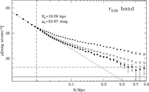
Fig. 6.18
The average light profile of 683 galaxy
clusters from the maxBCG catalog (Sect. 6.2.4) with
0. 2 ≤ z ≤ 0. 3. The
upper row of symbols
(triangles) show the total
light profile, the open
circles show the light profile after masking out identified
galaxies (except the central BCG). Since these are detectable only
up to some brightness limit, one can correct for this
incompleteness by statistically subtracting fainter galaxies, based
on an assumed luminosity function. This corrected brightness
profile is shown as filled
circles with error bars, which thus indicates the sum of the
BCG light profile plus the intracluster light. In the inner part,
this follows a de Vaucouleurs profile, indicated by the
dotted line, but
beyond ∼ 60 kpc there is clear excess of light, detected out to
almost 1 Mpc. Source: S. Zibetti et al. 2005, Intergalactic stars in z ∼ 0.25 galaxy
clusters: systematic properties from stacking of Sloan Digital Sky
Survey imaging data, MNRAS 358, 949, p. 957, Fig. 5.
Reproduced by permission of Oxford University Press on behalf of
the Royal Astronomical Society
Observation of
intracluster light. The observation of diffuse optical light
in clusters of galaxies and, related to this, the detection of the
intracluster stellar population, is extremely difficult. Although
first indications were already found with photographic plate
measurements, the surface brightness of this cluster component is
so low that even with CCD detectors the observation is
extraordinarily challenging. To quantify this, we note that the
surface brightness of this diffuse light component is about
30 mag arcsec−2 at a distance of several hundred kpc
from the cluster center. This value needs to be compared with the
brightness of the night sky, which is about
21 mag arcsec−2 in the V-band. One therefore needs to
correct for the effects of the night sky to better than a tenth of
a percent for the intergalactic stellar component to become visible
in a cluster. Furthermore, cluster galaxies and objects in the
foreground and background need to be masked out in the images, in
order to measure the radial profile of this diffuse component. This
is possible only up to a certain limiting magnitude, of course, up
to which individual objects can be identified. The existence of
weaker sources has to be accounted for with statistical methods,
which in turn use the luminosity function of galaxies. An example
of this ICL is shown in Fig. 6.17.
The identification of this diffuse optical light
as truly intergalactic origin is hampered by the fact that many
clusters host a central cD galaxy. As we mentioned in
Sect. 3.2.2 (see also Fig. 3.11), such galaxies have an
extended brightness profile with a surface brightness substantially
higher than the extrapolation of a de Vaucouleurs profile at large
radii. Thus the natural question arises whether the diffuse
component is just part of the cD envelope or a separate entity. If
the ICL belongs to the central galaxy, it should be gravitationally
bound to it; otherwise, it is a genuine intracluster component.
This issue can be investigated by kinematical observations of
individual stars in the ICL. One finds that the velocity dispersion
of the stars in the ICL strongly increases away from the central
galaxy, suggesting that they are unbound to it. One of the best
individual tracers of the ICL are planetary nebulae which are
formed in the final stages of Solar-mass stars. Since they emit a
large fraction of their energy in a single emission line, they are
ideal targets for spectroscopy. The kinematic study of
intergalactic planetary nebulae show that they are not part of the
central cluster galaxy. Related studies were carried out also with
red giant stars and globular clusters. Also, Type Ia supernovae
were found in clusters, but outside any cluster galaxy.
The diffuse light component was investigated in a
statistical superposition of the images of several galaxy clusters.
Statistical fluctuations in the sky background and uncertainties in
the flatfield6
determination are in this case averaged out. In this analysis an
 -law
is found for the light distribution in the inner region of
clusters, i.e., the (de Vaucouleurs) brightness profile of the
central galaxy is measured (see Fig. 6.18). For radii larger
than about ∼ 50 kpc, the brightness profile exceeds the
extrapolation of the de Vaucouleurs profile, and is detected out to
very large distances from the cluster center.
-law
is found for the light distribution in the inner region of
clusters, i.e., the (de Vaucouleurs) brightness profile of the
central galaxy is measured (see Fig. 6.18). For radii larger
than about ∼ 50 kpc, the brightness profile exceeds the
extrapolation of the de Vaucouleurs profile, and is detected out to
very large distances from the cluster center.The ICL is best studied in nearby groups and
clusters; only for them can individual objects be detected to a low
luminosity level. Furthermore, the cosmological surface brightness
dimming  (see problem 6.2) renders the detection
of ICL increasingly more difficult when turning to higher redshift.
Nevertheless, an ICL component was discovered out to redshift
z ∼ 0. 5, perhaps even as
far out as z ∼ 1. The
diffuse cluster component accounts for about 10 % of the total
optical light in a cluster; in some clusters this fraction can be
even higher. Therefore, models of galaxy evolution in clusters
should provide an explanation for these observations.
(see problem 6.2) renders the detection
of ICL increasingly more difficult when turning to higher redshift.
Nevertheless, an ICL component was discovered out to redshift
z ∼ 0. 5, perhaps even as
far out as z ∼ 1. The
diffuse cluster component accounts for about 10 % of the total
optical light in a cluster; in some clusters this fraction can be
even higher. Therefore, models of galaxy evolution in clusters
should provide an explanation for these observations.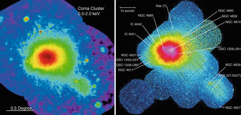
Fig. 6.19
X-ray images of the Coma cluster, taken
with the ROSAT-PSPC (left)
and XMM-EPIC (right). The
image size in the left
panel is 2. 7∘× 2. 5∘, much larger
than the optical image shown in Fig. 1.17. A remarkable feature is the
secondary maximum in the X-ray emission at the lower right of the
cluster center which shows that even Coma, long considered to be a
regular cluster, is not completely in an equilibrium state, but is
dynamically evolving, presumably by the accretion of a galaxy
group. Credit: left: S.L.
Snowden, NASA, GSFC; right:
U. Briel et al. 2001, A
mosaic of the Coma cluster of galaxies with XMM-Newton,
A&A 365, L60, p. L62, Fig. 1. ©ESO. Reproduced with
permission
6.4 Hot gas in galaxy clusters
One of the most important discoveries of the
UHURU X-ray satellite, launched in 1970, was the detection of X-ray
radiation from massive clusters of galaxies. With the later
Einstein X-ray satellite and more recently ROSAT, X-ray emission
was also detected from lower-mass clusters and groups. Three
examples for the X-ray emission of galaxy clusters are displayed in
Figs. 6.19,
6.20, and
6.21.
Figure 6.19 shows the Coma cluster of galaxies,
observed with two different X-ray observatories. Although Coma was
considered to be a fully relaxed cluster, distinct substructure is
visible in its X-ray radiation. The cluster RXJ 1347−1145
(Fig. 6.20)
is the most X-ray luminous cluster in the ROSAT All-Sky Survey
(Sect. 6.4.5). A large mass estimate of this cluster
also follows from the analysis of the gravitationally lensed arcs
(see Sect. 6.6) that are visible in Fig. 6.20; the cover of this
book shows a more recent image of this cluster, taken with the ACS
camera on-board HST, where a large number of arcs can be readily
detected. Finally, Fig. 6.21 shows a superposition of the X-ray
emission and an optical image of the cluster MS 1054−03, which is
situated at z = 0. 83 and
was for many years the highest redshift cluster known.
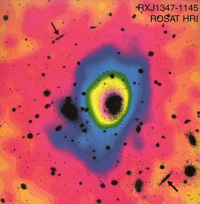
Fig. 6.20
RXJ 1347−1145 is one of the most luminous
galaxy clusters in the X-ray domain. A color-coded ROSAT/HRI image
of this cluster, which shows the distribution of the intergalactic
gas, is superposed on an optical image of the cluster with redshift
z = 0. 45. The two arrows indicate giant arcs, images
of background galaxies which are strongly distorted by the
gravitational lens effect. Credit: Max-Planck-Institut für
extraterrestrische Physik
6.4.1 General properties of the X-ray radiation
Clusters of galaxies are the brightest
extragalactic X-ray sources besides AGNs. If an X-ray telescope is
pointed away from the Galactic disk, about 85 % of the detected
sources are AGNs, the remaining ∼ 15 % are clusters. In contrast to
AGNs, for which the X-ray emission is essentially point-like, the
X-ray emission of clusters is extended. Their characteristic
luminosity is L
X ∼ 1043 erg∕s up to ∼ 1045 erg∕s
for the most massive systems. The fact that this X-ray emission is
spatially extended implies that it does not originate from
individual galaxies. The spatial region from which we can detect
this radiation can have a size of 1 Mpc or even larger. In
accordance with the extended nature of the X-ray source, no
variability of its X-ray flux has been detected.
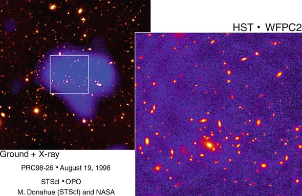
Fig. 6.21
The cluster of galaxies MS 1054−03 is, at
z = 0. 83, the
highest-redshift cluster in the Einstein Medium Sensitivity Survey,
which was compiled from observations with the Einstein satellite
(see Sect. 6.4.5). On the
right, an HST image of the cluster is shown, while
on the left is an optical
image, obtained with the 2.2-m telescope of the University of
Hawaii, superposed (in blue) with the X-ray emission of the
cluster measured with the ROSAT-HRI. Credit: Megan Donahue/STSCI,
Isabella Gioia/Univ. of Hawaii and NASA
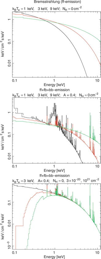
Fig. 6.22
X-ray emission of an optically thin hot
plasma. In the top panel,
the bremsstrahlung spectrum is shown, for three different gas
temperatures; the radiation of hotter gas extends to higher photon
energies, and above E ∼ k B T the spectrum is exponentially cut
off. In the central panel, atomic transitions and recombination
radiation in the hot gas are also taken into account, where a
metallicity of 40 % of the Solar value is assumed. These additional
radiation mechanisms become more important towards lower
T, as can be seen from the
T = 1 keV curve. In the
bottom panel,
photo-electric absorption by the Galactic interstellar medium is
included, with different column densities in hydrogen; for this
gas, Solar metallicity is assumed. The Galactic absorption produces
a cut-off in the spectrum towards lower energies. Credit: T.
Reiprich, Argelander-Institut für Astronomie, Universität
Bonn
Continuum
radiation. The spectral energy distribution of the X-rays
leads to the conclusion that the emission process is optically thin
thermal bremsstrahlung (free-free radiation) from a hot gas which
is collisionally ionized. This radiation is produced by the
acceleration of electrons in the Coulomb field of protons and
atomic nuclei. Since an accelerated electrically charged particle
emits radiation, such scattering processes between electrons and
protons in an ionized gas yields emission of photons. From the
spectral properties of this radiation, the gas temperature in
galaxy clusters can be determined, which is, for clusters with mass
between  and
and  , in the range of
107 K to 108 K, or 1 to 10 keV,
respectively.
, in the range of
107 K to 108 K, or 1 to 10 keV,
respectively.
and , in the range of
107 K to 108 K, or 1 to 10 keV,
respectively.The emissivity of bremsstrahlung is described by

(6.31)
where e
denotes the elementary charge, n e and n i the number density of
electrons and ions, respectively, Ze the charge of the ions, and
m e the electron
mass. The dimensionless function g ff is called Gaunt-factor;
it is a quantum mechanical correction factor of order 1, or, more
precisely,
 Hence, the spectrum described by (6.31) is flat for
 , and
exponentially decreasing for
, and
exponentially decreasing for  , as is
displayed in Fig. 6.22.
, as is
displayed in Fig. 6.22.
, and
exponentially decreasing for , as is
displayed in Fig. 6.22.The temperature of the gas in massive clusters is
typically T ∼ 5 ×
107 K, or k
B T ∼ 5 keV—X-ray astronomers usually
specify temperatures and frequencies in keV (see Appendix C).
For a thermal plasma with Solar abundances, the total
bremsstrahlung emission is

(6.32)
Line
emission. The assumption that the X-ray emission originates
from a hot, diffuse gas (intracluster medium, ICM) was confirmed by
the discovery of line emission in the X-ray spectrum of clusters.
One of the most prominent lines in massive clusters is located at
energies just below 7 keV: it is the Lyman-α (“Kα”) line of 25-fold ionized iron (thus,
of an iron nucleus with only a single electron). Slightly less
ionized iron has a strong transition at somewhat lower energies of
E ∼ 6. 4 keV. Later, other
lines were also discovered in the X-ray spectrum of clusters. As a
rule, the hotter the gas is, thus the more completely ionized it
is, the weaker the line emission. The X-ray emission of clusters
with relatively low temperatures, k B T ≲ 2 keV, is sometimes dominated by
line emission from highly ionized atoms (C, N, O, Ne, Mg, Si, S,
Ar, Ca, and a strong line complex of iron at E ∼ 1 keV—see Fig. 6.22). The emissivity of
a thermal plasma with Solar abundance and temperatures in the range
 can roughly be approximated by
 Equation (6.33) accounts for free-free emission as well
as line emission. Compared to (6.32), one finds a
different dependence on temperature: while the total emissivity for
bremsstrahlung is ∝ T
1∕2, it increases again towards lower temperatures where
the line emission becomes more important (see also
Fig. 10.3 for the temperature dependence
of the emissivity of a gas). It should be noted in particular that
the emissivity depends quadratically on the density of the plasma,
since both bremsstrahlung and the collisional excitation
responsible for line emission are two-body processes. Thus in order
to estimate the mass of the hot gas from its X-ray luminosity, the
spatial distribution of the gas needs to be known. For example, if
the gas in a cluster is locally inhomogeneous, the value of
Equation (6.33) accounts for free-free emission as well
as line emission. Compared to (6.32), one finds a
different dependence on temperature: while the total emissivity for
bremsstrahlung is ∝ T
1∕2, it increases again towards lower temperatures where
the line emission becomes more important (see also
Fig. 10.3 for the temperature dependence
of the emissivity of a gas). It should be noted in particular that
the emissivity depends quadratically on the density of the plasma,
since both bremsstrahlung and the collisional excitation
responsible for line emission are two-body processes. Thus in order
to estimate the mass of the hot gas from its X-ray luminosity, the
spatial distribution of the gas needs to be known. For example, if
the gas in a cluster is locally inhomogeneous, the value of
 which determines the X-ray emissivity may deviate significantly
from
which determines the X-ray emissivity may deviate significantly
from  . As
we will see later, clusters of galaxies satisfy a number of scaling
relations, and one relation between the gas mass and the X-ray
luminosity is found empirically, from which the gas mass can be
estimated. One finds that the mass in the intracluster gas is about
five to ten times larger than the mass of the stars in the
galaxies, where this ratio slightly increases with increasing
cluster mass.
. As
we will see later, clusters of galaxies satisfy a number of scaling
relations, and one relation between the gas mass and the X-ray
luminosity is found empirically, from which the gas mass can be
estimated. One finds that the mass in the intracluster gas is about
five to ten times larger than the mass of the stars in the
galaxies, where this ratio slightly increases with increasing
cluster mass.
can roughly be approximated by
(6.33)
which determines the X-ray emissivity may deviate significantly
from . As
we will see later, clusters of galaxies satisfy a number of scaling
relations, and one relation between the gas mass and the X-ray
luminosity is found empirically, from which the gas mass can be
estimated. One finds that the mass in the intracluster gas is about
five to ten times larger than the mass of the stars in the
galaxies, where this ratio slightly increases with increasing
cluster mass.Morphology of the
X-ray emission. From the morphology of their X-ray emission,
one can roughly distinguish between regular and irregular clusters,
as is also done in the classification of the galaxy distribution.
In Fig. 6.23,
X-ray surface brightness contours are superposed on optical images
of four galaxy clusters or groups, covering a wide range of cluster
mass and X-ray temperature. Regular clusters show a smooth
brightness distribution, centered on the optical center of the
cluster, and an outwardly decreasing surface brightness. In
contrast, irregular clusters may have several brightness maxima,
often centered on cluster galaxies or subgroups of cluster
galaxies.
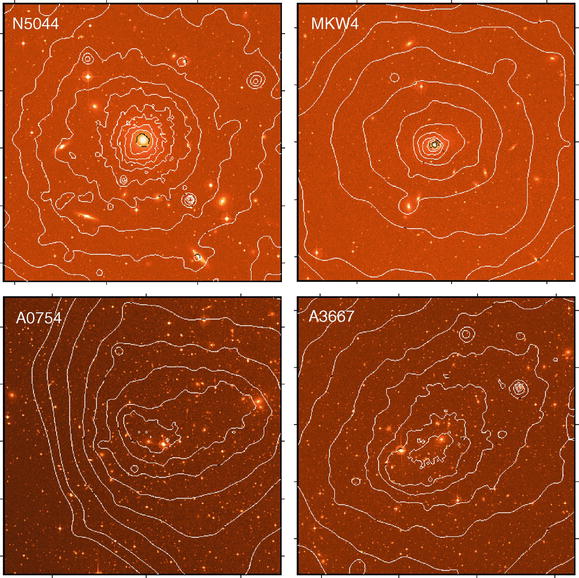
Fig. 6.23
Surface brightness contours of the X-ray
emission for four different groups or clusters of galaxies. Each
image is about 30 ′ on a side. Upper left: the galaxy group NGC 5044,
at redshift z = 0. 009,
with an X-ray temperature of T ≈ 1. 07 keV and a virial mass of
 .
Upper right: the group
MKW4, at z = 0. 02, with
T ≈ 1. 71 keV and
.
Upper right: the group
MKW4, at z = 0. 02, with
T ≈ 1. 71 keV and
 .
Lower left: the cluster of
galaxies A 0754, at z = 0. 053, with T ≈ 9. 5 keV and
.
Lower left: the cluster of
galaxies A 0754, at z = 0. 053, with T ≈ 9. 5 keV and  .
Lower right: the cluster of
galaxies A 3667, at z = 0. 056, with T ≈ 7. 0 keV and
.
Lower right: the cluster of
galaxies A 3667, at z = 0. 056, with T ≈ 7. 0 keV and  .
The X-ray data were obtained by ROSAT, and the optical images were
taken from the Digitized Sky Survey. These clusters are part of the
HIFLUGCS survey, which we will discuss more thoroughly in
Sect. 6.4.5.
Credit: T. Reiprich, Argelander-Institut für Astronomie,
Universität Bonn
.
The X-ray data were obtained by ROSAT, and the optical images were
taken from the Digitized Sky Survey. These clusters are part of the
HIFLUGCS survey, which we will discuss more thoroughly in
Sect. 6.4.5.
Credit: T. Reiprich, Argelander-Institut für Astronomie,
Universität Bonn
.
Upper right: the group
MKW4, at z = 0. 02, with
T ≈ 1. 71 keV and
.
Lower left: the cluster of
galaxies A 0754, at z = 0. 053, with T ≈ 9. 5 keV and .
Lower right: the cluster of
galaxies A 3667, at z = 0. 056, with T ≈ 7. 0 keV and .
The X-ray data were obtained by ROSAT, and the optical images were
taken from the Digitized Sky Survey. These clusters are part of the
HIFLUGCS survey, which we will discuss more thoroughly in
Sect. 6.4.5.
Credit: T. Reiprich, Argelander-Institut für Astronomie,
Universität BonnTypically, regular clusters have an X-ray
luminosity L X
and temperature that smoothly increases with cluster mass. In
contrast, irregular clusters at a given mass can be either hotter
or cooler than regular clusters. Irregular clusters are the result
of a recent merging event, and their temperature depends on the
stage of the merging process. In the initial phases of the merger,
the kinetic energy is not yet thermalized, and thus the gas remains
at approximately the same temperature it had before the merging
event. Later on, the gas is heated by shock fronts in which the
kinetic energy is transformed into internal energy of the gas—i.e.,
heat. In this phase, the gas temperature can be higher than that of
a regular cluster of the same mass. Finally, the cluster settles
into an equilibrium state. Indications of past merger events can be
seen in substructures of the X-ray emitting gas; even for the Coma
cluster, which is frequently considered a typical example of a
relaxed cluster, signs of previous merger events can be detected,
as shown in Fig. 6.24.
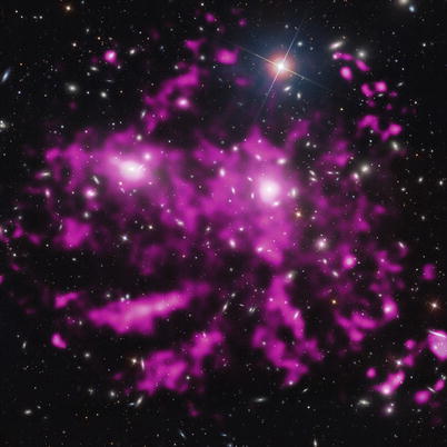
Fig. 6.24
In white, on optical image of the Coma
cluster is shown. Superposed on this SDSS image is the X-ray
emission, shown in pink,
where the smooth component of the X-ray image was subtracted to
highlight the filamentary structure of the hot gas. These filaments
are most likely due to a past merger events, when smaller groups
fall into the main cluster; their gas was stripped by ram-pressure
during infall, leaving trails of gas. The sidelength of the image
is 23 ′ ,
corresponding to about 600 kpc. Credit: X-ray: NASA/CXC/MPE/J.
Sanders et al., Optical: SDSS
The trend emerges that in clusters with a larger
fraction of spiral galaxies, L X and T are lower. Irregular clusters
typically also have a lower central density of galaxies and gas
compared to regular clusters. Clusters of galaxies with a dominant
central galaxy often show a strong central peak in X-ray emission.
The X-ray emission often deviates from axial symmetry, so that the
assumption of clusters being roughly spherically symmetric is not
well founded in these cases.
6.4.2 Models of the X-ray emission
Hydrostatic
assumption. To draw conclusions about the properties of the
intergalactic (intra-cluster) medium from the observed X-ray
radiation and about the distribution of mass in the cluster, the
gas distribution needs to be modeled. In fact, as we shall see
below, assuming the geometry of the cluster (e.g., spherical
symmetry), the radial dependence of the gas density can be directly
reconstructed. For this, we first consider the speed of sound in
the cluster gas,

where P
denotes the gas pressure, ρ
g the gas density, and n the number density of gas particles.
Then, the average molecular
mass is defined as the average mass of a gas particle in
units of the proton mass,
 so that
  .
For a gas of fully ionized hydrogen, one gets
.
For a gas of fully ionized hydrogen, one gets  because in this case one has one proton and one electron
per ∼ proton mass. The cluster gas also contains helium and heavier
elements; accounting for them yields μ ∼ 0. 60. The sound-crossing time for
the cluster is
because in this case one has one proton and one electron
per ∼ proton mass. The cluster gas also contains helium and heavier
elements; accounting for them yields μ ∼ 0. 60. The sound-crossing time for
the cluster is

(6.34)
.
For a gas of fully ionized hydrogen, one gets
because in this case one has one proton and one electron
per ∼ proton mass. The cluster gas also contains helium and heavier
elements; accounting for them yields μ ∼ 0. 60. The sound-crossing time for
the cluster is
and is thus, for a cluster with T ∼ 108 K, significantly
shorter than the lifetime of the cluster, which can be approximated
roughly by the age of the Universe. Since the sound-crossing time
defines the time-scale on which deviations from the pressure
equilibrium are evened out, the gas can be in hydrostatic
equilibrium, provided that the last major merging event happened
longer ago than the sound-crossing time. In this case, the equation

(6.35)
applies, with Φ denoting the gravitational potential.
Equation (6.35) describes how the gravitational force is
balanced by the pressure force. In the spherically symmetric case
in which all quantities depend only on the radius r, we obtain
 where M(r) is the mass enclosed within radius
r. Here, M(r) is the total enclosed mass, i.e.,
not just the gas mass, because the potential Φ is determined by the total mass. Note
the similarity of this equation with (6.9), except that there
P described the dynamical
pressure of the galaxies or dark matter particles. By inserting
where M(r) is the mass enclosed within radius
r. Here, M(r) is the total enclosed mass, i.e.,
not just the gas mass, because the potential Φ is determined by the total mass. Note
the similarity of this equation with (6.9), except that there
P described the dynamical
pressure of the galaxies or dark matter particles. By inserting
 into (6.36), we obtain

(6.36)
into (6.36), we obtain
(6.37)
This equation is of central importance for the
X-ray astronomy of galaxy clusters because it shows that we can
derive the mass profile M(r) from the radial profiles of
ρ g
and T. Thus, if one
can measure the density and temperature profiles, the mass of the
cluster, and hence the total density, can be determined as a
function of radius.
However, these measurements are not without
difficulties. ρ
g(r) and
T(r) need to be determined from the X-ray
luminosity and the spectral temperature, using the bremsstrahlung
emissivity (6.31). Obviously, they can be observed only in
projection in the form of the surface brightness
 from which the emissivity, and thus density and temperature, need
to be derived by de-projection, i.e., the inversion
of (6.38) to obtain ε ν (r) in terms of I ν (R). Furthermore, the angular and energy
resolution of X-ray telescopes prior to XMM-Newton and Chandra were
not high enough to measure both ρ g(r) and T(r) with sufficient accuracy, except for
the nearest clusters. For this reason, the mass determination was
often performed by employing additional, simplifying
assumptions.
from which the emissivity, and thus density and temperature, need
to be derived by de-projection, i.e., the inversion
of (6.38) to obtain ε ν (r) in terms of I ν (R). Furthermore, the angular and energy
resolution of X-ray telescopes prior to XMM-Newton and Chandra were
not high enough to measure both ρ g(r) and T(r) with sufficient accuracy, except for
the nearest clusters. For this reason, the mass determination was
often performed by employing additional, simplifying
assumptions.
(6.38)
Isothermal gas
distribution. From the radial profile of I(R), ε(r) can be derived by inversion
of (6.38). Since the spectral bremsstrahlung
emissivity depends only weakly on T for h P ν ≪ k B T—see (6.31)—the radial profile
of the gas density ρ
g can be derived from ε(r). The X-ray satellite ROSAT was
sensitive to radiation of  ,
so that the X-ray photons detected by it are typically from the
regime where h P
ν ≪ k B T.
,
so that the X-ray photons detected by it are typically from the
regime where h P
ν ≪ k B T.
,
so that the X-ray photons detected by it are typically from the
regime where h P
ν ≪ k B T.Assuming that the gas temperature is spatially
constant, T(r) = T g, (6.37) simplifies, and the
mass profile of the cluster can be determined from the density
profile of the gas.
The
β -model. A commonly used method consists
of fitting the X-ray data by a so-called β-model. This model is based on the
assumption that the density profile of the total matter (dark and
luminous) is described by an isothermal distribution, i.e., it is
assumed that the temperature of the gas is independent of radius,
and at the same time that the mass distribution in the cluster is
described by the isothermal model that was discussed in
Sect. 6.3.1.
With (6.9) and (6.12), we then obtain for
the total density ρ(r)
 On the other hand, in the isothermal case (6.37) reduces to
 The comparison of (6.39) and (6.40) then shows that
 ,
or
,
or
![$$\displaystyle{ \rho _{\mathrm{g}}(r) \propto \left [\rho (r)\right ]^{\beta }\quad \mathrm{with}\quad \fbox{$\beta:= \frac{\mu m_{\mathrm{p}}\sigma _{v}^{2}} {k_{\mathrm{B}}T_{\mathrm{g}}}$} }$$](A129044_2_En_6_Chapter_Equ41.gif) must apply; thus the gas density follows the total density to some
power. Here, the index β
depends on the ratio of the dynamical temperature, measured by
σ v , and the gas temperature. Now,
using the King approximation for an isothermal mass
distribution—see (6.17)—as a model for the mass distribution, we
obtain
must apply; thus the gas density follows the total density to some
power. Here, the index β
depends on the ratio of the dynamical temperature, measured by
σ v , and the gas temperature. Now,
using the King approximation for an isothermal mass
distribution—see (6.17)—as a model for the mass distribution, we
obtain
![$$\displaystyle{ \fbox{$\rho _{\mathrm{g}}(r) =\rho _{\mathrm{g0}}\left [1 + \left ( \frac{r} {r_{\mathrm{c}}}\right )^{2}\right ]^{-3\beta /2}$}\;, }$$](A129044_2_En_6_Chapter_Equ42.gif) where ρ g0 is
the central gas density. The brightness profile of the X-ray
emission in this model is then, according to (6.38),
where ρ g0 is
the central gas density. The brightness profile of the X-ray
emission in this model is then, according to (6.38),
![$$\displaystyle{ \fbox{$I(R) \propto \left [1 + \left ( \frac{R} {r_{\mathrm{c}}}\right )^{2}\right ]^{-3\beta +1/2}$}\;. }$$](A129044_2_En_6_Chapter_Equ43.gif)
(6.39)
(6.40)
,
or
(6.41)
(6.42)
(6.43)
The X-ray emission of many clusters is well
described by this profile,7 yielding values for r c of 0. 1 to
0. 3h −1 Mpc and
a value for the index β = β fit ≈ 0. 65.
Alternatively, β can be
measured, with the definition given in (6.41), from the gas
temperature T g
and the velocity dispersion of the galaxies σ v , which yields typical values
of β = β spec ≈ 1. Such a value
would also be expected if the mass and gas distributions were both
isothermal. In this case, they should have the same temperature,
which was presumably determined by the formation of the
cluster.
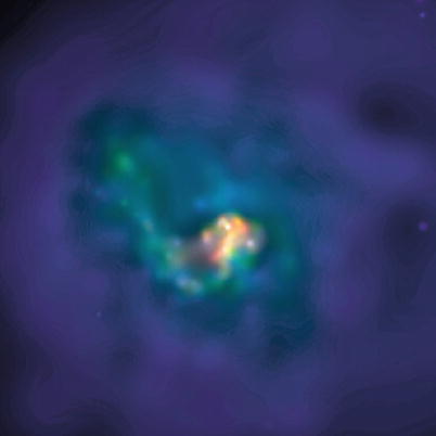
Fig. 6.25
Chandra image of the Centaurus cluster; the
size of the field is 3 ′ × 3 ′ . Owing to the excellent
angular resolution of the Chandra satellite, the complexity of the
morphology in the X-ray emission of clusters can be analyzed.
Colors indicate photon
energies, from low to high in red, yellow, green, and blue. The gas in the center of the
cluster is significantly cooler than that at larger radii. Credit:
NASA/IoA/J. Sanders & A. Fabian
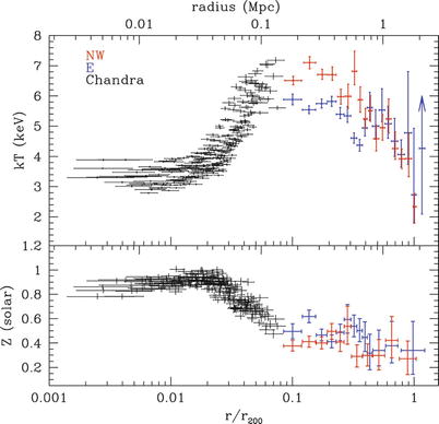
Fig. 6.26
Temperature (top) and metallicity (bottom) profile of the Perseus cluster,
measured along two different directions from the cluster center
outwards. Black symbols
show measurements in the inner region, obtained with Chandra. The
colored points are obtained
from Suzaku data, with each color corresponding to one radial
direction. Source: A. Simionescu et al. 2011, Baryons at the Edge of the X-ray-Brightest
Galaxy Cluster, Science 331, 1576, Fig. 2. Reprinted with
permission from AAAS
The
β -discrepancy. The fact that the two
values for β determined above differ from
each other (the so-called β-discrepancy) is almost certainly due
to the fact that the β-model is too simple. We can see,
e.g., from Fig. 6.25 that the gas distribution, at least in the
inner part of clusters, does not follow a smooth distribution, nor
is its temperature constant. The latter is also reflected by the
fact that the measured values for β fit often depend on the
angular range over which the brightness profile is fitted: the
larger this range, the larger β fit becomes, and thus the
smaller the discrepancy. This behavior can be understood if the
central region of the clusters have a lower temperature than at
larger radii. Furthermore, temperature measurements of clusters are
often not very accurate because it is the emission-weighted
temperature which is measured, which is, due to the quadratic
dependence of the emissivity on ρ g, dominated by the
regions with the highest gas density. The fact that the innermost
regions of clusters where the gas density is highest tend to have a
temperature below the bulk temperature of the cluster (see
Fig. 6.26)
may lead to an underestimation of ‘the’ cluster temperature. In
addition, the near independence of the spectral form of
 from T for h P ν ≪ k B T renders the measurement of
T difficult. Chandra and
XMM-Newton can measure the X-ray emission at energies of up to
E ≲ 10 keV, which resulted
in considerably improved temperature determinations.
from T for h P ν ≪ k B T renders the measurement of
T difficult. Chandra and
XMM-Newton can measure the X-ray emission at energies of up to
E ≲ 10 keV, which resulted
in considerably improved temperature determinations.
from T for h P ν ≪ k B T renders the measurement of
T difficult. Chandra and
XMM-Newton can measure the X-ray emission at energies of up to
E ≲ 10 keV, which resulted
in considerably improved temperature determinations.Such investigations have revealed that the
temperature behavior shown in Fig. 6.26 is typical for many
clusters: The temperature decreases towards the center and towards
the edge, while it is rather constant over a larger range at
intermediate radii. Many clusters are found, however, in which the
temperature distribution is by no means radially symmetric, but
shows distinct substructure. Finally, as another possible
explanation for the β-discrepancy, it should be mentioned
that the velocity distribution of those galaxies from which
σ v is measured may be
anisotropic.
Besides all the uncertainty as to the validity of
the β-model, we also need
to mention that numerical simulations of galaxy clusters, which
take dark matter and gas into account, have repeatedly come to the
conclusion that the mass determination of clusters, utilizing the
β-model, should achieve an
accuracy of better than ∼ 20 %, although different gas dynamical
simulations have arrived at distinctly different results.
Dark matter in
clusters from X-ray observations. Based on measurements of
their X-ray emission, a mass estimate can be performed for galaxy
clusters. It is found, in agreement with the dynamical method, that
clusters contain much more mass than is visible in galaxies. The
total mass of the intergalactic medium is clearly too low to
account for the missing mass; its gas mass is only ∼ 15 % of the
total mass of a cluster.
Only ∼ 3 % of the mass in
clusters of galaxies is due to stars in galaxies, and about 15% is
contributed by the intergalactic gas, whereas the remaining ∼ 80 %
consists of dark matter which therefore dominates the mass of the
clusters.
6.4.3 Cooling “flows”
Expected
consequences of gas cooling. In examining the intergalactic
medium, we assumed hydrostatic equilibrium, but we disregarded the
fact that the gas cools by its emission and by that loses internal
energy. For this reason, once established, a hydrostatic
equilibrium in principle cannot be maintained over arbitrarily long
times. To decide whether this gas cooling is important for the
dynamics of the system, the cooling time-scale needs to be
considered. This cooling time turns out to be very long,
 where
where  is the
energy density of the gas and n e the electron density.
Hence, the cooling time is longer than the Hubble time nearly
everywhere in the cluster, which allows a hydrostatic equilibrium to be established to
a very good approximation. In the centers of clusters, however, the
density may be sufficiently large to yield
is the
energy density of the gas and n e the electron density.
Hence, the cooling time is longer than the Hubble time nearly
everywhere in the cluster, which allows a hydrostatic equilibrium to be established to
a very good approximation. In the centers of clusters, however, the
density may be sufficiently large to yield  .
Here, the gas can cool quite efficiently, by which its pressure
decreases. This then implies that, at least close to the center,
the hydrostatic equilibrium can no longer be maintained. To
re-establish pressure equilibrium, gas needs to flow inwards and is
thus compressed. Hence, an inward-directed mass flow should
establish itself. The corresponding density increase will further
accelerate the cooling process. Since, in addition, the
emissivity (6.33) of a relatively cool gas increases with
decreasing temperature, this process should then very quickly lead
to a strong compression and cooling of the gas in the centers of
dense clusters. It is a process which, once started, will
accelerate and quickly lead to the cooling down to very low
temperatures. In parallel to this increase in density, the X-ray
emission should strongly increase, because
.
Here, the gas can cool quite efficiently, by which its pressure
decreases. This then implies that, at least close to the center,
the hydrostatic equilibrium can no longer be maintained. To
re-establish pressure equilibrium, gas needs to flow inwards and is
thus compressed. Hence, an inward-directed mass flow should
establish itself. The corresponding density increase will further
accelerate the cooling process. Since, in addition, the
emissivity (6.33) of a relatively cool gas increases with
decreasing temperature, this process should then very quickly lead
to a strong compression and cooling of the gas in the centers of
dense clusters. It is a process which, once started, will
accelerate and quickly lead to the cooling down to very low
temperatures. In parallel to this increase in density, the X-ray
emission should strongly increase, because  .
As a result of this process, a radial density and temperature
distribution should be established with a nearly unchanged pressure
distribution. In Fig. 6.25, the cooler gas in the center of the
Centaurus cluster is clearly visible.
.
As a result of this process, a radial density and temperature
distribution should be established with a nearly unchanged pressure
distribution. In Fig. 6.25, the cooler gas in the center of the
Centaurus cluster is clearly visible.
(6.44)
is the
energy density of the gas and n e the electron density.
Hence, the cooling time is longer than the Hubble time nearly
everywhere in the cluster, which allows a hydrostatic equilibrium to be established to
a very good approximation. In the centers of clusters, however, the
density may be sufficiently large to yield .
Here, the gas can cool quite efficiently, by which its pressure
decreases. This then implies that, at least close to the center,
the hydrostatic equilibrium can no longer be maintained. To
re-establish pressure equilibrium, gas needs to flow inwards and is
thus compressed. Hence, an inward-directed mass flow should
establish itself. The corresponding density increase will further
accelerate the cooling process. Since, in addition, the
emissivity (6.33) of a relatively cool gas increases with
decreasing temperature, this process should then very quickly lead
to a strong compression and cooling of the gas in the centers of
dense clusters. It is a process which, once started, will
accelerate and quickly lead to the cooling down to very low
temperatures. In parallel to this increase in density, the X-ray
emission should strongly increase, because .
As a result of this process, a radial density and temperature
distribution should be established with a nearly unchanged pressure
distribution. In Fig. 6.25, the cooler gas in the center of the
Centaurus cluster is clearly visible.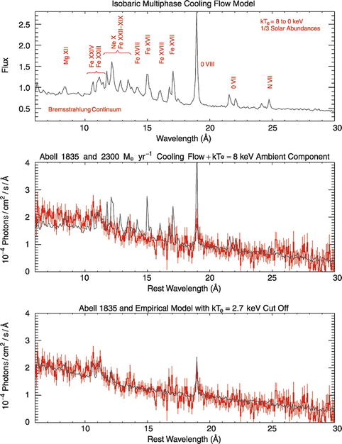
Fig. 6.27
In the top
panel, a model spectrum of a cooling flow is shown, in which
the gas cools down from 8 keV to T g = 0. The strong lines of
Fexvii can be seen. In
the central panel, the
spectrum of Abell 1835 is superposed on the model spectrum; clear
discrepancies are visible, especially the absence of strong
emission lines from Fexvii. If the gas is not allowed to
cool down to temperatures below 3 keV (bottom panel), the agreement with
observation improves visibly. Source: J.R. Peterson et al.
2003, High Resolution X-ray
Spectroscopic Constraints on Cooling-Flow Models,
astro-ph/0310008, Fig. 2. Reproduced by permission of the
author
Some predictions of this so-called cooling flow model have indeed been
verified observationally. In the centers of many massive clusters,
one observes a sharp central peak in the surface brightness
I(R). However, we need to stress that, as
yet, no inwards flows have
been measured. Such a measurement would be very difficult, though,
due to the small expected velocities. The amount of cooling gas can
be considerable. We can estimate the mass rate  at
which the gas should cool and flow inwards due to this cooling. The
internal energy U of the
gas is related to its mass M by
at
which the gas should cool and flow inwards due to this cooling. The
internal energy U of the
gas is related to its mass M by  , with u as given above. The loss of this
energy due to cooling is the luminosity,
, with u as given above. The loss of this
energy due to cooling is the luminosity,  ,
so that
,
so that
 For some massive clusters, this estimate lead to cooling rates of
tens or even hundreds of Solar masses per year. However, after
spectroscopic observations by XMM-Newton became available, we have
learned that these very high cooling rates implied by the models
were significantly
overestimated.
For some massive clusters, this estimate lead to cooling rates of
tens or even hundreds of Solar masses per year. However, after
spectroscopic observations by XMM-Newton became available, we have
learned that these very high cooling rates implied by the models
were significantly
overestimated.
at
which the gas should cool and flow inwards due to this cooling. The
internal energy U of the
gas is related to its mass M by , with u as given above. The loss of this
energy due to cooling is the luminosity, ,
so that
(6.45)
The fate of the
cooling gas. The gas cooling in this way will accumulate in
the center of the cluster, but despite the expected high mass of
cold gas, no clear evidence has been found for it. In clusters
harboring a cD galaxy, the cooled gas may, over a Hubble time,
contribute a considerable fraction of the mass of this galaxy.
Hence, the question arises whether cD galaxies may have formed by
accretion in cooling flows. In this scenario, the gas would be
transformed into stars in the cD galaxy. However, the
star-formation rate in these central galaxies is much lower than
the rate by which cluster gas cools, according to the ‘old’ cooling
flow models sketched above.

Fig. 6.28
The cool-core cluster Abell 2597 at
z = 0. 082. The
upper left panel shows the
Chandra X-ray map as green contours, superposed on an optical image
of the brightest cluster galaxy (BCG) of this cluster. Note that
the overall orientation of the X-ray emission follows that of the
light in the BCG. Upper
right: The color map is obtained from subtracting a smoothed
version of the X-ray emission from the one shown in the
left panel; this so-called
‘unsharp mask’ image highlights the small-scale brightness
variations. Superposed on this are radio contours at three
different frequencies, increasing from green to blue to black. Clearly,
the BCG contains an active nucleus, and the radio jet apparently
causes an X-ray cavity on the right of the galaxy center. The
lower left panel shows the
temperature map, as obtained from resolved X-ray spectroscopy, with
the total X-ray emission superposed. The temperature in the inner
part is markedly smaller than at larger radii, a clear sign of a
cool core. Note also the small-scale structure in the temperature
map. The spectral energy distribution of the core, shown at the
lower right, yields a clear
indication of ongoing star formation, seen from the far-IR
radiation due to warm dust. Further indications for ongoing star
formation is obtained from the UV-radiation, as well as emission
lines of the object (not shown). Source: Upper and lower right panels: G.R. Tremblay
et al. 2012, Residual cooling
and persistent star formation amid active galactic nucleus feedback
in Abell 2597, MNRAS 424, 1042, p. 1046, 1053, Figs. 1,
4. Lower left panel: G.R. Tremblay et al. 2012, Multiphase signatures of active galactic
nucleus feedback in Abell 2597, MNRAS 424, 1026,
p. 1036, Fig. 7. Reproduced by permission of Oxford University
Press on behalf of the Royal Astronomical Society
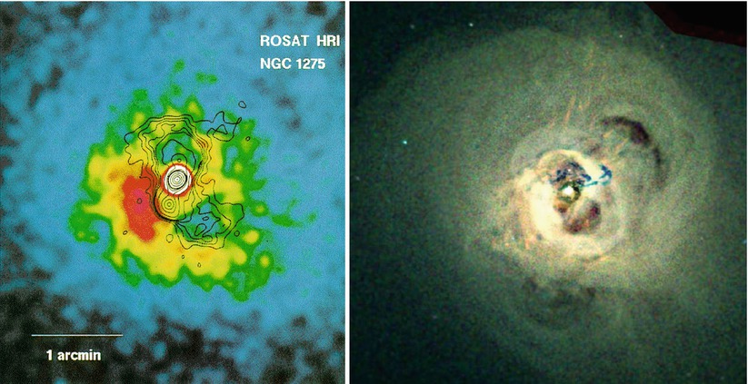
Fig. 6.29
The central region of the Perseus cluster.
The left panel shows a
color-coded X-ray image, taken with ROSAT, with radio contours
superposed. The radio emission stems from the central galaxy of the
cluster, the radio galaxy NGC 1275 (also called Perseus A). Clearly
identifiable is the effect of the radio jets on the X-ray
emission—at the location of the radio lobes the X-ray emission is
strongly suppressed. The right
panel shows a slightly larger region in X-rays, taken with
the considerably better resolution of Chandra. The fine structure
of the X-ray gas is much better recognized here. In addition to the
two cavities overlapping with the radio emission, another pair of
bubbles at larger distance from the center is seen. The high X-ray
luminosity and small distance from us allows a very detailed
analysis of this cluster. In particular, sound waves in the X-ray
gas can be identified which probably are due to earlier activity of
the central black hole. The blue filaments near the center
indicates hard X-ray emission; the hardening of the observed
spectrum is due to an infalling galaxy at high velocity, whose
interstellar medium absorbs the low-energy X-ray photons. Credit:
Left: H. Böhringer, MPE.
Right:
NASA/CXC/IoA/A. Fabian et al.
The absence of
massive cooling flows. The sensitivity and spectral
resolution achieved with XMM-Newton have strongly modified our view
of cooling flows. In the standard model of cooling flows, the gas
cools from the cluster temperature down to temperatures
significantly below 1 keV. In this process many atomic lines are
emitted, produced by various ionization stages, e.g., of iron,
which strongly depend on temperature. Figure 6.27 (top panel) shows
the expected spectrum of a cooling flow in which the gas cools down
from the cluster temperature of T g ≈ 8 keV to essentially
T g = 0, where a
chemical composition of 1/3 Solar abundance is assumed. In the
central panel, this theoretical spectrum is compared with the
spectrum of the cluster Abell 1835, where very distinct
discrepancies become visible. In the bottom panel, the model was
modified such that the gas cools down only to T g = 3 keV; this model
clearly matches the observed spectrum better.
Hence, cooler gas in the inner regions of
clusters is directly detected spectroscopically. However, the
temperature measurements from X-ray spectroscopy are significantly
different from the prediction of the cooling flow model according
to which drastic cooling should take place in the gas, because the
process of compression and cooling will accelerate for ever
decreasing T g.
Therefore, one expects to find gas at all temperatures lower than
the temperature of the cluster. But this seems not to be the case:
whereas the central temperature can be considerably smaller than
that at larger radii (see, e.g., Fig. 6.26), no gas seems to be
present at very small temperatures, although the cooling flow model
predicts the existence of such gas. A minimum temperature seems to
exist, below which the gas cannot cool, or the amount of gas that
cools to T g ∼ 0
is considerably smaller than expected from the cooling flow model.
This lower mass rate of gas that cools down completely would then
also be compatible with the observed low star-formation rates in
the central galaxies of clusters. In fact, a correlation between
the cooling rate of gas as determined from XMM observations and the
regions of star formation in clusters has been found (see
Fig. 6.28).
About 50 % of X-ray luminous clusters show an infrared excess of
the BCG, indicating ongoing star formation; furthermore, whereas
the BCG in clusters with long cooling time rarely show optical
emission lines, most of those in cooling flow clusters do. All
these are clear indications that a few percent of the cooling mass
rate (6.45) as estimated from the cooling flow model
indeed arrive at the central cluster galaxy.
There may be exceptional cases where a larger
fraction of the cooling gas can reach the gravitational center of
the cluster and cool down to low temperatures. Recently, a cluster
at z ∼ 0. 6 was discovered
with an extremely large cooling mass rate  where the
BCG shows signs of massive star formation, estimated to be
where the
BCG shows signs of massive star formation, estimated to be
 . Such cases are
rare, however, and may be a transitional state in the cluster
evolution.
. Such cases are
rare, however, and may be a transitional state in the cluster
evolution.
where the
BCG shows signs of massive star formation, estimated to be
. Such cases are
rare, however, and may be a transitional state in the cluster
evolution.
Fig. 6.30
A composite X-ray (blue, taken by Chandra) and radio
(pink, VLA) image of the
galaxy cluster Abell 400. The radio jets are launched by a binary
supermassive black hole in the center of the galaxy NGC 1128, also
known as 3C 75, a wide angle tailed radio source. The energy of the
jets is partly transferred to the hot intracluster medium, which is
thereby heated. The strong curvature of the jets is caused by the
relative motion of the galaxy through the ICM, i.e., the jets are
‘pushed back’ by ram pressure. With a (projected) separation of
about 8 kpc, this is one of the closest supermassive black hole
binary system known. Credit: X-ray: NASA/CXC/AIfA/D. Hudson &
T. Reiprich et al.; Radio: NRAO/VLA/NRL
Cool-core
clusters. Not all clusters show indications for a cool inner
region with a strongly peaked X-ray emission. If clusters are
far from an equilibrium state, for example due to a recent merger
or infall of a group, the gas will be far from a quasi-steady
state, and the foregoing consideration will not apply, not even
approximately. Strong mixing of the gas by turbulent motions, or
shock fronts which develop when the intracluster medium of two
colliding or merging clusters intersect, will prevent the
development of a cool, condensed central region. One thus
distinguishes between cool-core
clusters and non-cool-core clusters. The former ones are
expected to be close to hydrostatic equilibrium, whereas the latter
ones may deviate from it strongly.
What prevents
massive cooling flows? One way to explain the clearly
suppressed cooling rates in cooling flows is by noting that many
clusters of galaxies harbor an active galaxy in their center. In
most cases, this AGN is not a luminous quasar, but radio galaxies
are the most common type of AGNs in the BCG of clusters, the
activity of which, e.g., in the form of (radio-)jets, may affect
the ICM. For instance, energy could be transferred from the jet to
the ICM, by which the ICM is heated. This heating might then
prevent the temperature from dropping to arbitrarily small values.
This hypothesis is supported by the fact that many clusters are
known in which the ICM is clearly affected by the central AGN—see
Fig. 6.29 for
one of the first examples where this effect was seen, and
Fig. 6.30
where two active nuclei are detected. In the cluster Abell 2597
shown in Fig. 6.28 the interaction of the radio source with
the intracluster gas is also clearly seen. Plasma from the jet
seems to locally displace the X-ray emitting gas. By friction and
mixing in the interface region between the jet and the ICM, the
latter is certainly heated. It is unclear, though, whether this
explanation is valid for every cluster, because not every cluster
in which a very cool ICM is expected also contains an observed AGN.
On the other hand, this is not necessarily an argument against the
hypothesis of AGNs as heating sources, since AGNs often have a
limited time of activity and may be switching on and off, depending
on the accretion rate. Thus, the gas in a cluster may very well be
heated by an AGN even if it is currently (at the time of
observation) inactive. Evidence for the occurrence of this effect
also in galaxy groups is shown in Fig. 6.31.
Fig. 6.31
Galaxy groups are also X-ray emitters,
albeit weaker than clusters of galaxies. Moreover, the temperature
of the ICM is lower than in clusters. This 4 ′ × 4 ′ Chandra image shows HCG 62.
Note the complexity of the X-ray emission and the two symmetrically
aligned regions that seem to be virtually devoid of hot
ICM—possibly holes blown free by jets from the central galaxy of
this group (NGC 4761). Credit: NASA/CfA/J. Vrtilek
et al.
Two more examples of the impact of a central AGN
on the cluster gas are shown in Fig. 6.32. The energetics of
this interaction can be enormous, as can be seen in the cluster
MS 0735.6+7421 shown in the right panel of Fig. 6.32. The large size of
the cavities in the X-ray emitting gas implies that a huge amount
of energy was needed to push the gas away. From the cavity size and
the gas density, one estimates that about  of gas has been displaced,
requiring an energy of about 1062 erg. If this energy
was generated by accretion onto the supermassive black hole located
in the central galaxy of the cluster, with a mass-to-energy
conversion of 10 %, the mass of the SMBH has grown by
of gas has been displaced,
requiring an energy of about 1062 erg. If this energy
was generated by accretion onto the supermassive black hole located
in the central galaxy of the cluster, with a mass-to-energy
conversion of 10 %, the mass of the SMBH has grown by  . Assuming that the
gas was removed with about the sound speed of the ICM, this energy
was released in the past ∼ 108 yr, implying a mean
luminosity of the central AGN of ∼ 3 × 1046 erg∕s of
mechanical energy. Hence, by all accounts, this is a very energetic
event which strongly impacts on the ICM of this cluster.
. Assuming that the
gas was removed with about the sound speed of the ICM, this energy
was released in the past ∼ 108 yr, implying a mean
luminosity of the central AGN of ∼ 3 × 1046 erg∕s of
mechanical energy. Hence, by all accounts, this is a very energetic
event which strongly impacts on the ICM of this cluster.
of gas has been displaced,
requiring an energy of about 1062 erg. If this energy
was generated by accretion onto the supermassive black hole located
in the central galaxy of the cluster, with a mass-to-energy
conversion of 10 %, the mass of the SMBH has grown by . Assuming that the
gas was removed with about the sound speed of the ICM, this energy
was released in the past ∼ 108 yr, implying a mean
luminosity of the central AGN of ∼ 3 × 1046 erg∕s of
mechanical energy. Hence, by all accounts, this is a very energetic
event which strongly impacts on the ICM of this cluster.Feedback.
The heating of the intracluster medium by a central radio source in
clusters is the most visible example of feedback. We will encounter other
examples lateron when we discuss the evolution of galaxies. As the
gas cools and sinks towards the center, the central supermassive
black hole can get fresh fuel and starts producing energy. The
corresponding energy output in form of kinetic power in the radio
jets or in radiation then heats the gas again, preventing efficient
cooling and thus limits the mass accretion rate—and thus the
fueling of the AGN. Hence, one might have a feedback loop, which
does not need to have a stable equilibrium. The mass accretion rate
may vary in time, as well as the AGN power output. Most likely, the
feedback loop is somewhat more complicated than depicted here, but
there is no doubt that AGN feedback is essential for understanding
the gas in galaxy clusters.
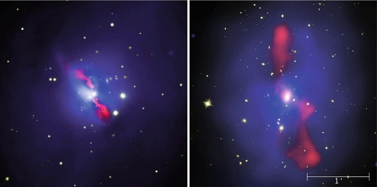
Fig. 6.32
The left
panel shows the galaxy cluster Hydra A at redshift
z = 0. 054. This composite
image is 4.′8 on the side and shows the X-ray emission
(blue) and radio emission
(red) superposed on the
optical image. Clearly seen is the impact of the radio jets on the
intracluster gas—at the location of the jets, the X-ray emission is
strongly suppressed, whereas around the radio jets, overdensities
are visible. Here, the gas, which has been pushed away from the
jet, is accumulated. The right
panel shows a composite image of the galaxy cluster
MS 0735.6+7421 with redshift z = 0. 216, showing the inner 700 kpc
(corresponding to 200 ′
′ ) of the cluster. The Chandra X-ray image is shown
in blue, and the radio
emission as seen by the VLA shown in red, both superposed on an optical HST
image of the cluster. The X-ray emission displays large cavities,
located right at the position where the radio jets pass through the
intracluster medium. This cluster contains presumably the most
energetic interaction of the central AGN with the intracluster
medium. Credit: Left:
X-ray: NASA/CXC/U.Waterloo/C. Kirkpatrick et al.; Radio:
NSF/NRAO/VLA; Optical: Canada-France-Hawaii-Telescope/DSS.
Right: NASA, ESA, CXC,
STScI, and B. McNamara (University of Waterloo), NRAO, and L.
Birzan and team (Ohio University); journal article: B.R. McNamara
et al. 2009, An Energetic AGN
Outburst Powered by a Rapidly Spinning Supermassive Black Hole or
an Accreting Ultramassive Black Hole, ApJ 698, 594,
p. 595, Fig. 1 ©AAS. Reproduced with permission
Wide angle tail
radio galaxies. Radio galaxies in clusters often have a
different radio morphology than isolated ones. The radio jets
necessarily interact with the intracluster gas and will be affected
by it. Correspondingly, if the radio galaxy has a significant
velocity relative to the ICM, the shape of the jets will get bend
by ram pressure. A typical example for such wide angle tail radio source is shown
in Fig. 6.33.
Radio sources with such strong bended jets essentially only occur
in clusters. Therefore, such sources can be used to search for
clusters, and indeed these cluster searches have been successful—up
to redshifts of order unity.
The Bullet
cluster. Clusters of galaxies are indeed excellent
laboratories for hydrodynamical and plasma-physics processes on
large scales. Shock fronts, for instance in merging clusters,
cooling fronts (which are also called ‘contact discontinuities’ in
hydrodynamics), and the propagation of sound waves can be observed
in their intracluster medium. A particularly good example is
the galaxy cluster 1E 0657−56 displayed in Fig. 6.34, also called the
‘Bullet cluster’. To the right of the cluster center, strong and
relatively compact X-ray emission (the ‘bullet’) is visible, while
further to the right of it one sees an arc-shaped
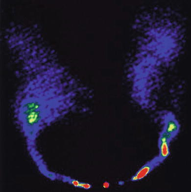
Fig. 6.33
NGC 1265, a radio galaxy in the Perseus
cluster. Owing to its motion through the intracluster gas, with an
estimated velocity of ∼ 2000 km∕s, its radio jets get bend by ram
pressure. Credit: Image courtesy of NRAO/AUI and C. O’Dea & F.
Owen
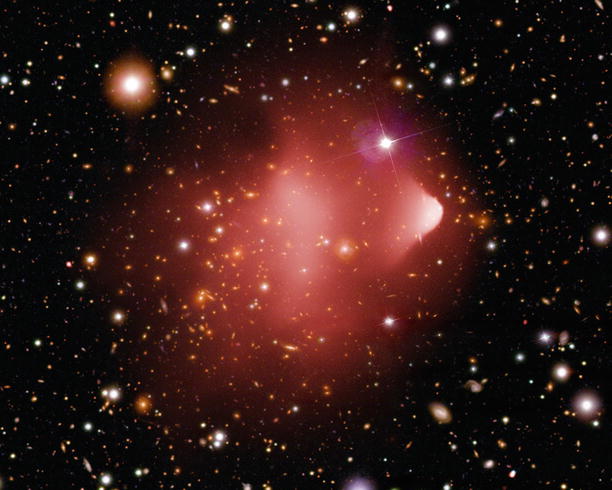
Fig. 6.34
The cluster of galaxies 1E 0657−56 is a
perfect example of a merging cluster. The X-ray emission of this
cluster as observed by Chandra, shown in red, is superposed on an optical HST
image. The most remarkable feature in the X-ray map is the compact
region to the right (westwards) of the cluster center (from which
the cluster derives its name the ‘Bullet cluster’), and the sharp
transition in the surface brightness further at its right edge. An
analysis of the brightness profile and of the X-ray temperature
distribution shows that this must be a shock front moving at about
2.5 times the speed of sound, or v ∼ 3500 km∕s, through the gas. To the
right of this shock front, a group of galaxies is visible. Credit:
X-ray: NASA/CXC/CfA/M. Markevitch et al.; Optical: NASA/STScI;
Magellan/U.Arizona/D. Clowe et al.
discontinuity in surface brightness. From the
temperature distribution on both sides of the discontinuity one
infers that it is a shock front—in fact, the shape of the gas
distribution on the right resembles that of the air around a
supersonic plane or bullet. The strength of the shock implies that
the ‘bullet’ is moving at about v ∼ 3500 km∕s through the intergalactic
medium of the cluster. The interpretation of this observation is
that we are witnessing the collision of two clusters, where one
less massive cluster has passed, from left to right in
Fig. 6.34,
through a more massive one. The ‘bullet’ in this picture is
understood to be gas from the central region of the less massive
cluster, which is still rather compact. This interpretation is
impressively supported by the group of galaxies to the right of the
shock front, which are probably the former member galaxies of the
less massive cluster. As this cluster crosses through the more
massive one, its galaxies and dark matter are moving
collisionlessly, whereas the gas is decelerated by friction with
the gas in the massive cluster: the galaxies and the dark matter
are thus able to move faster through the cluster than the gas,
which is lagging behind (and whose momentum transferred to the gas
of the more massive cluster displaces the latter from its original
location, centered on the corresponding galaxy distribution). We
will see below that this interpretation is verified by a
gravitational lens investigation of this double cluster.
Fig. 6.35
The influence of the Sunyaev–Zeldovich
effect on the cosmic background radiation. The dashed curve represents the Planck
distribution of the unperturbed CMB spectrum, the solid curve shows the spectrum after
the radiation has passed through a cloud of hot electrons. The
magnitude of this effect, for clarity, has been very much
exaggerated in this sketch. Source: J. Carlstrom et al. 2002,
ARA&A 40, 643, Fig. 1, p. 646. Reprinted, with permission,
from the Annual Review of
Astronomy & Astrophysics, Volume 40 ©2002 by Annual
Reviews www.annualreviews.org
Fig. 6.36
Maps of the nearby cluster Abell 2319 in
seven frequencies, obtained by the Planck satellite. These maps
(with about 2∘ sidelength) clearly indicate the
Sunyaev–Zeldovich effect caused by the hot gas in this cluster. At
low frequencies, the SZ-effect causes a decrease of the surface
brightness, whereas at high frequencies, the intensity is
increased. The transition between these two regimes occurs at
218 GHz, as shown in Fig. 6.35; indeed, in the map of this frequency, no
signal is seen. Credit and Copyright: ESA/LFI & HFI
Consortia
6.4.4 The Sunyaev–Zeldovich effect
Electrons in the hot gas of the intracluster
medium can scatter photons of the cosmic microwave background. The
optical depth and thus the scattering probability for this Compton
scattering is relatively low, but the effect is nevertheless
observable and, in addition, is of great importance for the
analysis of clusters, as we will now see.
Spectral
signature. A photon moving through a cluster of galaxies
towards us will change its direction through scattering and thus
will not reach us. But since the cosmic background radiation is
isotropic, for any CMB photon that is scattered out of the
line-of-sight, another photon exists—statistically—that is
scattered into it, so that the total number of photons reaching us
is preserved. However, the energy of the photons changes slightly
through scattering by the hot electrons, in a way that they have an
(on average) higher frequency after scattering. Hence, by this
inverse Compton scattering (Sect. 5.4.4),
energy is on average transferred from the electrons to the photons,
as can be seen in Fig. 6.35.
As a consequence, this scattering leads to a
reduced number of photons at lower energies, relative to the Planck
spectrum, which are shifted to higher energy. There is one photon
energy where the intensity is unchanged, corresponding to a
frequency of 218 GHz; below that frequency, the intensity is lower
than that of the CMB, for higher frequencies, the intensity is
increased. This effect is called the Sunyaev–Zeldovich effect (SZ-effect).
It was predicted in 1970 and has now been observed in a large
number of clusters. One example is presented in Fig. 6.36, where the frequency
dependence of the effect is clearly seen.
The CMB spectrum, measured in
the direction of a galaxy cluster, deviates from a Planck spectrum;
the degree of this deviation depends on the temperature of the
cluster gas and on its density, and is independent of the cluster
redshift.
In the Rayleigh–Jeans domain of the CMB spectrum,
at wavelengths larger than about 2 mm, the intensity of the CMB is
decreased by the SZ-effect. For the change in specific intensity in
the RJ part, one obtains
 where
where
 is the Compton-y parameter
and σ T the
Thomson cross section for electron scattering. Obviously,
y is proportional to the
optical depth with respect to Compton scattering, given as an
integral over n
e σ T
along the line-of-sight. Furthermore, y is proportional to the gas
temperature, because that defines the average energy transfer per
scattering event [see (5.35)]. Overall, y is proportional to the integral over
the gas pressure P = nk B T g along the line-of-sight
through the cluster.
is the Compton-y parameter
and σ T the
Thomson cross section for electron scattering. Obviously,
y is proportional to the
optical depth with respect to Compton scattering, given as an
integral over n
e σ T
along the line-of-sight. Furthermore, y is proportional to the gas
temperature, because that defines the average energy transfer per
scattering event [see (5.35)]. Overall, y is proportional to the integral over
the gas pressure P = nk B T g along the line-of-sight
through the cluster.
(6.46)
(6.47)
Fig. 6.37
Left: The Sunyaev–Zeldovich effect of
the Coma cluster, as seen by the Planck satellite. The microwave
temperature depletion is color coded, whereas the white contours
display the X-ray emission of the cluster as measured by ROSAT.
Both maps are superposed on the optical image from the Digitized
Sky Survey 2. Note the very close correspondence between the
SZ-signal and the X-ray emission. Right: The cluster SPT-CL J2106−5844
was detected by its SZ-signal, which is shown here as contour
lines, superposed on a composite optical and mid-IR image, taken
with the Magellan telescope and the Spitzer observatory,
respectively. The cluster has a redshift of z = 1. 13, and is (one of) the most
massive clusters at redshift z > 1, with an estimated virial mass
of  . The
cluster is also detected in X-rays, showing a very high temperature
of T ∼ 11 keV, and an X-ray
luminosity of L
X ∼ 1. 4 × 1045 erg∕s. The image is 4
′ 8 on the side.
Encircled galaxies have their cluster membership spectroscopically
confirmed. Credit and Copyright: Left: Planck image: ESA/LFI & HFI
Consortia; ROSAT image: Max-Planck-Institut für extraterrestrische
Physik; DSS image: NASA, ESA, and the Digitized Sky Survey.
Acknowledgment: Davide De Martin (ESA/Hubble). Right: R.J. Foley et al. 2011,
Discovery and Cosmological
Implications of SPT-CL J2106−5844, the Most Massive Known Cluster
at z > 1, ApJ 731, 86, p. 3, Fig. 1. ©AAS.
Reproduced with permission
. The
cluster is also detected in X-rays, showing a very high temperature
of T ∼ 11 keV, and an X-ray
luminosity of L
X ∼ 1. 4 × 1045 erg∕s. The image is 4
′ 8 on the side.
Encircled galaxies have their cluster membership spectroscopically
confirmed. Credit and Copyright: Left: Planck image: ESA/LFI & HFI
Consortia; ROSAT image: Max-Planck-Institut für extraterrestrische
Physik; DSS image: NASA, ESA, and the Digitized Sky Survey.
Acknowledgment: Davide De Martin (ESA/Hubble). Right: R.J. Foley et al. 2011,
Discovery and Cosmological
Implications of SPT-CL J2106−5844, the Most Massive Known Cluster
at z > 1, ApJ 731, 86, p. 3, Fig. 1. ©AAS.
Reproduced with permission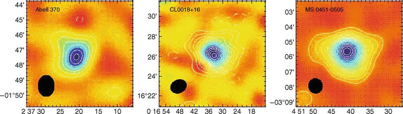
Fig. 6.38
Sunyaev–Zeldovich maps of three clusters of
galaxies at 0. 37 < z < 0. 55. Plotted is the
temperature difference of the measured CMB relative to the average
CMB temperature (or, at fixed frequency, the difference in
radiation intensities). The black ellipse in each image specifies
the instrument’s beam size. For each of the clusters shown here,
the spatial dependence of the SZ-effect is clearly visible. Since
the SZ-effect is proportional to the electron density, the mass
fraction of baryons in clusters can be measured if one additionally
knows the total mass of the cluster from dynamical methods or from
the X-ray temperature. The analysis of the clusters shown here
yields for the mass fraction of the intergalactic gas f g ≈ 0. 08 h −1. Source: L. Grego
et al. 2001, Galaxy Cluster
Gas Mass Fractions from Sunyaev-Zeldovich Effect Measurements:
Constraints on Ω m, ApJ 552, 2, p. 7,
Fig. 1. ©AAS. Reproduced with permission
The fact that the SZ-signal Δ I ν ∕I ν is independent of cluster
redshift allows the investigation of clusters at high redshifts,
provided the SZ-signal is spatially resolved. As we will see below,
the SZ-effect can also be used to detect clusters in the first
place, and this selection is much less biased to low redshifts than
for flux-limited optical or X-ray surveys. As an example, the
right-hand panel of Fig. 6.37 shows a very massive, high-redshift
cluster that was selected by an SZ-survey.
Observations of the SZ-effect provide another
possibility for analyzing the gas in clusters. For instance, if one
can spatially resolve the SZ-effect, which is possible today with
interferometric methods (see Fig. 6.38), one obtains
information about the spatial density and temperature distribution.
Here it is of crucial importance that the dependence on temperature
and gas density is different from that in X-ray emission. Because
of the quadratic dependence of the X-ray emissivity on n e, the X-ray luminosity
depends not only on the total gas mass, but also on its spatial
distribution. Small-scale clumps in the gas, for instance, would
strongly affect the X-ray emission. In contrast, the SZ-effect is
linear in gas density and therefore considerably less sensitive to
small-scale inhomogeneities in the ICM.
The integrated
y-parameter. The amplitude of the spectral distortion caused
by the SZ-effect is given by y, and SZ-maps essentially provide a
map of y as a function of
angular position in the cluster. When integrating y across the cluster, we get the total
SZ-signal,
 hence, the integrated SZ-effect is proportional to the integrated
SZ-parameter
hence, the integrated SZ-effect is proportional to the integrated
SZ-parameter
 We see that Y is a measure
of the product of gas mass and temperature. Both of these
quantities can also be determined from X-ray observations, so that
an independent estimate of Y can be obtained. In order to
distinguish between the two, one usually denotes the result from
SZ-observations by Y
SZ, in contrast to Y X when it is determined
from X-ray studies. These two can be different in general, due to
the quadratic dependence of the X-ray emission on local gas density
or through the temperature variation inside clusters.
We see that Y is a measure
of the product of gas mass and temperature. Both of these
quantities can also be determined from X-ray observations, so that
an independent estimate of Y can be obtained. In order to
distinguish between the two, one usually denotes the result from
SZ-observations by Y
SZ, in contrast to Y X when it is determined
from X-ray studies. These two can be different in general, due to
the quadratic dependence of the X-ray emission on local gas density
or through the temperature variation inside clusters.
(6.48)
(6.49)
Kinetic
SZ-effect. Beside the thermal SZ-effect just described,
there is a related effect, called the kinetic SZ-effect. This is
due to the fact that clusters may have a peculiar velocity. Suppose
the peculiar velocity of a cluster is directed towards us, then the
photons scattering in its intracluster gas and reaching us will be
scattered by electrons which have an average velocity towards us.
These scattered photons thus experience on average a blueshift,
which is visible in the CMB spectrum in the direction of this
cluster. The kinetic SZ-effect has a different spectral signature
than the thermal SZ-effect and can thus in principle be
distinguished from it. A robust measurement of the kinetic
SZ-effect would allow a direct measurement of the line-of-sight
component of the peculiar velocities of clusters. However, the
expected amplitude of the kinetic SZ-effect is smaller than that of
the thermal SZ-effect by a factor of ∼ 10 and thus much harder to
detect. First detections have recently been reported in the
literature.
Distance
determination. For a long time, the SZ-effect was mainly
considered a tool for measuring distances to clusters of galaxies,
and from this to determine the Hubble constant. We will now
schematically show how the SZ-effect, in combination with the X-ray
emission, allows us to determine the distance to a cluster. The
change in the CMB intensity has the dependence
 where L is the extent of
the cluster along the line-of-sight. To obtain this relation, we
replace the l-integration
in (6.47) by a multiplication with L, which yields the correct functional
dependence. On the other hand, the surface brightness of the X-ray
radiation behaves as
where L is the extent of
the cluster along the line-of-sight. To obtain this relation, we
replace the l-integration
in (6.47) by a multiplication with L, which yields the correct functional
dependence. On the other hand, the surface brightness of the X-ray
radiation behaves as
 Combining these two relations, we are now able to eliminate
n e. Since
T g is
measurable from the X-ray spectrum, the dependence
Combining these two relations, we are now able to eliminate
n e. Since
T g is
measurable from the X-ray spectrum, the dependence
 remains. Now assuming that the cluster is spherical, its extent
L along the line-of-sight
equals its transverse extent R = θ
D A, where θ denotes its angular extent and
D A the
angular-diameter distance (4.49) to the cluster. With this
assumption, we obtain
remains. Now assuming that the cluster is spherical, its extent
L along the line-of-sight
equals its transverse extent R = θ
D A, where θ denotes its angular extent and
D A the
angular-diameter distance (4.49) to the cluster. With this
assumption, we obtain
 Hence, the angular-diameter distance can be determined from the
measured SZ-effect, the X-ray temperature of the ICM, and the
surface brightness in the X-ray domain. Of course, this method is
more complicated in practice than sketched here, but it is applied
to the distance determination of clusters. In particular, the
assumption of the same extent of the cluster along the
line-of-sight as its transverse size is not well justified for any
individual cluster due to triaxiality, but one expects this
assumption to be valid on average for a sample of clusters. Hence,
the SZ-effect is another method of distance determination,
independent of the redshift of the cluster, and therefore suitable
for determining the Hubble constant.
Hence, the angular-diameter distance can be determined from the
measured SZ-effect, the X-ray temperature of the ICM, and the
surface brightness in the X-ray domain. Of course, this method is
more complicated in practice than sketched here, but it is applied
to the distance determination of clusters. In particular, the
assumption of the same extent of the cluster along the
line-of-sight as its transverse size is not well justified for any
individual cluster due to triaxiality, but one expects this
assumption to be valid on average for a sample of clusters. Hence,
the SZ-effect is another method of distance determination,
independent of the redshift of the cluster, and therefore suitable
for determining the Hubble constant.
(6.50)
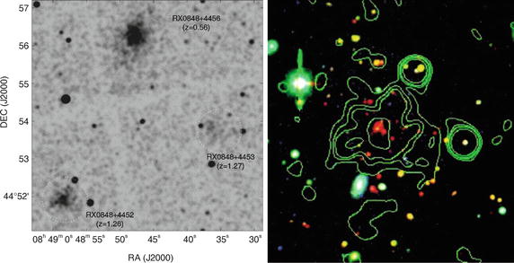
Fig. 6.39
On the
left: Chandra image of a 6 ′ × 6 ′ -field with two clusters of
galaxies at high redshift. On the
right: a 2 ′ × 2 ′ -field centered on one of the
clusters presented on the left (RX J0849+4452), in B, I, and K,
overlaid with the X-ray brightness contours. Source: S.A. Stanford
et al. 2001, The Intracluster
Medium in z > 1 Galaxy Clusters, ApJ 552, 504,
p. 505, 507, Figs. 1, 3. ©AAS. Reproduced with
permission
Discussion.
The natural question arises whether this method, in view of the
assumptions it is based on, can compete with the determination of
the Hubble constant via the distance ladder and Cepheids, as
described in Sect. 3.9, or from the CMB, to be
discussed in Sect. 8.7. The same question also needs to
be asked for the determination of H 0 by means of the time
delay in gravitational lens systems, which we discussed in
Sect. 3.11.4. In both cases, the answer
is the same: presumably neither of the two methods will provide a
determination of the Hubble constant with an accuracy comparable to
that achieved by the local methods and from the angular
fluctuations in the CMB. Nevertheless, both methods are of great
value for cosmology: first, the distance ladder has quite a number
of rungs. If only one of these contains an as yet undetected severe
systematic error, it could affect the resulting value for
H 0. Second, the
Hubble Key Project measured the expansion rate in the local
Universe, typically within ∼ 100 Mpc (the distance to the Coma
cluster). As we will see later, the Universe contains
inhomogeneities on these length scales. Thus, it may well be that
we live in a slightly overdense or underdense region of the
Universe, where the Hubble constant deviates from the global value.
In contrast to this, both the SZ-effect and the lensing method
measure the Hubble constant on truly cosmic scales, and both
methods do so in only a single step—there is no distance ladder
involved. For these reasons, these two methods are of considerable
interest in additionally confirming our H 0 measurements. Another
aspect adds to this, which must not be underestimated: even if the
same or a similar value results from these measurements as the one
from the Hubble Key Project, we still have learned an important
fact, namely that the local Hubble constant agrees with the one
measured on cosmological scales—as predicted by our cosmological
model, which can thus be tested. Indeed, both methods have been
applied to quite a number of lens systems and luminous clusters
showing an SZ effect, respectively, and they yield values for
H 0 which are
compatible within the error bars with the value of H 0 obtained from the Hubble
Key Project.
6.4.5 X-ray and SZ catalogs of clusters
As we have seen, projection effects may play a
crucial role in the selection of galaxy clusters through searching
for an overdensity of galaxies on the sphere using optical methods.
A more reliable way of selecting clusters is by their X-ray
emission, since the hot X-ray gas signifies a deep potential well,
thus a real three-dimensional overdensity of matter, so that
projection effects become virtually negligible. The X-ray emission
is  , which again renders
projection effects improbable. In addition, the X-ray emission, its
temperature in particular, seems to be a very good measure for the
cluster mass, as we will discuss further below. Whereas the
selection of clusters is not based on their temperature, but on the
X-ray luminosity, we shall see that L X is also a good indicator
for the mass of a cluster (see Sect. 6.5).
, which again renders
projection effects improbable. In addition, the X-ray emission, its
temperature in particular, seems to be a very good measure for the
cluster mass, as we will discuss further below. Whereas the
selection of clusters is not based on their temperature, but on the
X-ray luminosity, we shall see that L X is also a good indicator
for the mass of a cluster (see Sect. 6.5).
Fig. 6.40
The top
panel shows the total exposure time in the ROSAT All-Sky
Survey as a function of sky position. Near the ecliptic poles the
exposure time is longest, as a consequence of the applied observing
strategy. Because of the “South Atlantic Anomaly” (a region of
enhanced cosmic ray flux over the South Atlantic Ocean, off the
coast of Brazil, caused by the shape of the Earth’s magnetosphere),
the exposure time is generally higher in the North than in the
South. The X-ray sky, as observed in the RASS, is shown in the
lower panel. The colors
indicate the shape of the spectral energy distribution, where
blue indicates sources with
a harder spectrum. Credit: Max-Planck-Institut für
Extraterrestrische Forschung, Garching; journal article: S.L.
Snowden et al. 1997, ROSAT
Survey Diffuse X-Ray Background Maps. II., ApJ
485, 125
Fig. 6.41
Distribution of clusters in redshift and
mass, as obtained from three different surveys. Green points show clusters selected
through their X-ray emission, here from the ROSAT All-Sky Survey
(see Fig. 6.40). The crosses show clusters selected by their
SZ-signal, as obtained from the South Pole Telescope; its high
angular resolution resolves the SZ-signal even for very distant
clusters. Correspondingly, the mass distribution of the selected
cluster does not show any marked redshift dependence, at least out
to z ∼ 1. Red points show clusters selected by
Planck, also through their SZ-signal. Due to the lower angular
resolution of Planck, the signal from higher-redshift clusters,
which are smaller than the telescope beam, is diluted. Source: C.L.
Reichardt et al. 2013, Galaxy
Clusters Discovered via the Sunyaev-Zel’dovich Effect in the First
720 Square Degrees of the South Pole Telescope Survey, ApJ
763, 127, Fig. 4. ©AAS. Reproduced with permission
The first cosmologically interesting X-ray
catalog of galaxy clusters was the EMSS (Extended Medium
Sensitivity Survey) catalog. It was constructed from archival
images taken by the Einstein
observatory which were scrutinized for X-ray sources other
than the primary target in the field-of-view of the respective
observation. These were compiled and then further investigated
using optical methods, i.e., photometry and spectroscopy. The EMSS
catalog contains 835 sources, most of them AGNs, but it also
contains 104 clusters of galaxies. Among these are six clusters at
redshift ≥ 0. 5; the most distant is MS 1054−03 at z = 0. 83 (see Fig. 6.21). Since the Einstein
images all have different exposure times, the EMSS is not a
strictly flux-limited catalog. But with the flux limit known for
each exposure, the luminosity function of clusters can be derived
from this.
The same method as was used to compile the EMSS
was applied to ROSAT archival images by various groups, leading to
several catalogs of X-ray-selected clusters. The selection criteria
of the different catalogs vary. Since ROSAT was more sensitive than
the Einstein observatory, these catalogs contain a larger number of
clusters, and also ones at higher redshift (Fig. 6.39). Furthermore, ROSAT
performed a survey of the full sky, the ROSAT All-Sky Survey
(RASS). The RASS contains about 105 sources distributed
over the whole sky. The identification of extended sources in the
RASS (in contrast to non-extended sources—about five times more
AGNs than clusters are expected) yielded a catalog of clusters
which, owing to the relatively short exposure times in the RASS,
contains the brightest clusters. The exposure time in the RASS is
not uniform over the sky since the applied observing strategy led
to particularly long exposures for the regions around the Northern
and Southern ecliptic pole (see Fig. 6.40).
From the luminosity function of X-ray clusters, a
mass function can be constructed, using the relation between
L X and the
cluster mass that will be discussed in the following section.
Furthermore, as we will explain in more detail in
Sect. 8.2, this cluster mass function is
an important probe for cosmological parameters.
More recently, the sensitivity and throughput of
SZ telescopes and instruments became sufficiently large to not only
study the SZ-effect of known clusters, but to survey the sky for SZ
sources. In 2009 the first SZ-selected clusters were found, and at
the time of writing, at least three telescopes are used for
constructing cluster catalogs through SZ-selection. The South Pole
Telescope (SPT), the Atacama Cosmology Telescope, and the Planck
satellite, together have found more than 1000 clusters. The
selection criteria for SZ clusters is quite different from those of
X-ray (or optical) cluster samples, since we have seen that the
strength of the SZ-signal is redshift-independent, as long as the
cluster is spatially resolved. If, however, the angular resolution
of the observations is not high enough to resolve the SZ-signal
from a cluster, distant clusters are more difficult to find, since
the signal gets diluted. On the other hand, the SZ-signal is weak,
so that only the more massive clusters can be readily discovered.
The different selection effects are clearly visible in the redshift
and mass distribution of the resulting cluster catalogs, shown in
Fig. 6.41.
The fact that Planck finds the more massive clusters at redshifts
z ≲ 0. 5 originates from
its all-sky survey, in which the rare objects are found, whereas
the SPT clusters in Fig. 6.41 were selected from a region of
720 deg2.
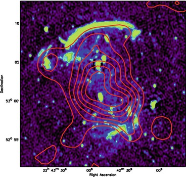
Fig. 6.42
1. 4 GHz map of the galaxy cluster CIZA
J2242.8+5301 at redshift z = 0. 1921, taken with the Westerbork
Synthesis Radio Telescope (WSRT), on which the X-ray contours
(shown in red) are
superposed. The most prominent radio source is the large elongated
feature some 1. 5 Mpc to the North of the cluster center, whose
length is ∼ 2 Mpc. Source: R.J. van Weeren et al. 2010,
arXiv:1010.4306, Fig. 1. Reproduced by permission of the
author
6.4.6 Radio relics
In some galaxy clusters, one finds extended,
diffuse radio sources at large cluster-centric radii, the so-called
radio relics. These radio sources do not coincide with member
galaxies in the cluster, and thus have an intracluster origin.
Their shapes are often very elongated or irregular, as can be seen
by the example shown in Fig. 6.42. The strong polarization of the radio
emission shows that the origin of the radiation is synchrotron
emission. Therefore, these radio relics must contain relativistic
electrons. About 50 radio relics have been found to date.
As we discussed in Sect. 5.1.3, relativistic particles are
accelerated in shock fronts, such as occur in supernova remnants.
Shock fronts are formed in plasmas with supersonic flow velocities.
A natural way of explaining the occurrence of a shock in the
outskirts of a cluster is to assume that the cluster has been
subject to a recent merger event. If the intracluster gas of the
two clusters run into each other, a shock front is formed. For the
radio relic shown in Fig. 6.42, the predictions of the shock hypothesis
were tested in quite some detail. The radio spectral index
α varies strongly across
the relic, from α ≈ 0. 6 to
about 2.0, indicating that the electron distribution closest to the
shock has the flattest spectrum, whereas it continuously steepens
away from the shock, due to energy losses. The high degree of
polarization ( ∼ 50 %) shows the presence of a very well-ordered
magnetic field in the emission region.
The merging hypothesis for the example shown in
Fig. 6.42 is
further supported by the strongly disturbed morphology of the
intracluster gas, as shown by the X-ray contours, as well as by the
indication of a second relic on the opposite side of the cluster
center; such counter relics are predicted from numerical
simulations of cluster mergers.
6.5 Scaling relations for clusters of galaxies
Our examination of galaxies revealed the
existence of various scaling relations, for example the
Tully–Fisher relation. These have proven to be very useful not only
for the distance determination of galaxies, but also because any
successful model of galaxy evolution needs to be able to explain
these empirical scaling relations—they must contain information
about the formation of galaxies. Therefore, it is of great interest
to examine whether clusters of galaxies also fulfill any such
scaling relation. As we will see, the X-ray properties of clusters
play a central role in this.
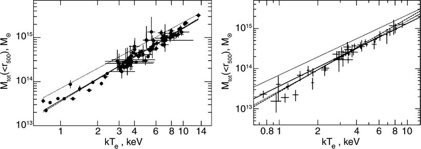
Fig. 6.43
For the clusters of galaxies from the
extended HIFLUGCS sample, the mass within a mean overdensity of 500
is plotted as a function of X-ray temperature, where a
dimensionless Hubble constant of h = 0. 5 was assumed. In the
left-hand panel, the mass
was determined by applying an isothermal β-model, while in the right-hand panel, the radial
temperature profile T(r) was used to determine the mass, by
means of (6.37). Most of the temperature measurements are
from observations by the ASCA satellite. The solid and dash-dotted curves in the left-hand panel show the best fit to
the data, where for the latter only the clusters from the original
HIFLUGCS sample were used. In the right-hand panel, the dashed line is a fit to all the data in
the plot, while the solid
line takes into account only clusters with a mass
 . In both panels,
the upper dotted line shows
the mass-temperature relation that was obtained from a simulation
using simplified gas dynamics—the slope agrees with that found from
the observations, but the amplitude is significantly too high.
Source: A. Finoguenov et al. 2001, Details of the mass-temperature relation for
clusters of galaxies, A&A 368, 749, p. 752,
Figs. 1, 2. ©ESO. Reproduced with permission
. In both panels,
the upper dotted line shows
the mass-temperature relation that was obtained from a simulation
using simplified gas dynamics—the slope agrees with that found from
the observations, but the amplitude is significantly too high.
Source: A. Finoguenov et al. 2001, Details of the mass-temperature relation for
clusters of galaxies, A&A 368, 749, p. 752,
Figs. 1, 2. ©ESO. Reproduced with permission6.5.1 Mass-temperature relation
It is expected that the larger the spatial
extent, velocity dispersion of galaxies, temperature of the X-ray
gas, and luminosity of a cluster are, the more massive it is. In
fact, from theoretical considerations one can deduce the existence
of relations between these parameters. The X-ray temperature
T specifies the thermal
energy per gas particle, which should be proportional to the
binding energy for a cluster in virial equilibrium,
 Since this relation is based on the virial theorem, r should be chosen to be the radius
within which the matter of the cluster is virialized. This value
for r is called the
virial radius r
vir. From theoretical considerations of cluster
formation (see Chap. 7), one finds that the virial radius
is defined such that within a sphere of radius r vir, the average mass
density of the cluster is about Δ c ≈ 200 times as high as
the critical density ρ
cr of the Universe (see also Problem 6.1). The mass within
r vir is called
the virial mass M
vir which is, according to this definition,
Since this relation is based on the virial theorem, r should be chosen to be the radius
within which the matter of the cluster is virialized. This value
for r is called the
virial radius r
vir. From theoretical considerations of cluster
formation (see Chap. 7), one finds that the virial radius
is defined such that within a sphere of radius r vir, the average mass
density of the cluster is about Δ c ≈ 200 times as high as
the critical density ρ
cr of the Universe (see also Problem 6.1). The mass within
r vir is called
the virial mass M
vir which is, according to this definition,
 Combining the two above relations, one obtains
 This relation can now be observationally tested by using a sample
of galaxy clusters with known temperature and with mass determined
by the methods discussed in Sect. 6.4.2. An example of this
is displayed in Fig. 6.43, in which the mass is plotted versus
temperature for clusters from the extended HIFLUGCS sample.8 Since it is easier to
determine the mass inside a smaller radius than the virial mass
itself, the mass M
500 within the radius r 500, the radius within
which the average density is 500 times the critical density, is
plotted here. The measured values clearly show a very strong
correlation, and best-fit straight lines describing power laws of
the form M = AT α are also shown in the figure.
The exact values of the two fit parameters depend on the choice of
the cluster sample; the right-hand panel of Fig. 6.43 shows in particular
that galaxy groups (thus, ‘clusters’ of low mass and temperature)
are located below the power-law fit that is obtained from higher
mass clusters. If one confines the sample to clusters with
This relation can now be observationally tested by using a sample
of galaxy clusters with known temperature and with mass determined
by the methods discussed in Sect. 6.4.2. An example of this
is displayed in Fig. 6.43, in which the mass is plotted versus
temperature for clusters from the extended HIFLUGCS sample.8 Since it is easier to
determine the mass inside a smaller radius than the virial mass
itself, the mass M
500 within the radius r 500, the radius within
which the average density is 500 times the critical density, is
plotted here. The measured values clearly show a very strong
correlation, and best-fit straight lines describing power laws of
the form M = AT α are also shown in the figure.
The exact values of the two fit parameters depend on the choice of
the cluster sample; the right-hand panel of Fig. 6.43 shows in particular
that galaxy groups (thus, ‘clusters’ of low mass and temperature)
are located below the power-law fit that is obtained from higher
mass clusters. If one confines the sample to clusters with
 , the best fit is
described by
, the best fit is
described by
 with an uncertainty in the parameters of slightly more than 10 %.
This relation is very similar to the one deduced from our
theoretical consideration, M ∝ T 1. 5. With only small
variations in the parameters, the relation (6.53) is obtained both
from a cluster sample in which the mass was determined based on an
isothermal β-model, and
from a cluster sample in which the measured radial temperature
profile T(r) was utilized in the mass
determination [see (6.37)]. Constraining the sample to clusters
with temperatures above 3 keV, one obtains a slope of 1. 48 ± 0. 1,
in excellent agreement with theoretical expectations. Considerably
steeper mass-temperature relations result from the inclusion of
galaxy groups into the sample, from which we conclude that they do
not follow in detail the scaling argument sketched above.
with an uncertainty in the parameters of slightly more than 10 %.
This relation is very similar to the one deduced from our
theoretical consideration, M ∝ T 1. 5. With only small
variations in the parameters, the relation (6.53) is obtained both
from a cluster sample in which the mass was determined based on an
isothermal β-model, and
from a cluster sample in which the measured radial temperature
profile T(r) was utilized in the mass
determination [see (6.37)]. Constraining the sample to clusters
with temperatures above 3 keV, one obtains a slope of 1. 48 ± 0. 1,
in excellent agreement with theoretical expectations. Considerably
steeper mass-temperature relations result from the inclusion of
galaxy groups into the sample, from which we conclude that they do
not follow in detail the scaling argument sketched above.
(6.51)
(6.52)
, the best fit is
described by
(6.53)
The X-ray temperature of galaxy
clusters apparently provides a very accurate measure for their
virial mass, better than the velocity dispersion (see below).
6.5.2 Mass-velocity dispersion relation
The velocity dispersion of the galaxies in a
cluster also can be related to the mass: from (6.26) we find
 Together with
  and
and  , it then follows
that
, it then follows
that
 This relation can now be tested using clusters for which the mass
was determined using the X-ray method, and for which measurements
of the velocity dispersion of the cluster galaxies are available.
Alternatively, the relation T ∝ σ v 2 can be tested. One
finds that these relations are essentially satisfied for the
observed clusters. However, the relation between σ v and M is not as tight as the M-T relation. Furthermore, numerous
clusters exist which strongly deviate from this relation. These are
clusters of galaxies that are not relaxed, as can be deduced from
the velocity distribution of the cluster galaxies (which strongly
deviates from a Maxwell distribution in these cases) or from a
bimodal or even more complex galaxy distribution in the cluster.
These outliers need to be identified, and removed, if one intends
to apply the scaling relation between mass and velocity
dispersion.
This relation can now be tested using clusters for which the mass
was determined using the X-ray method, and for which measurements
of the velocity dispersion of the cluster galaxies are available.
Alternatively, the relation T ∝ σ v 2 can be tested. One
finds that these relations are essentially satisfied for the
observed clusters. However, the relation between σ v and M is not as tight as the M-T relation. Furthermore, numerous
clusters exist which strongly deviate from this relation. These are
clusters of galaxies that are not relaxed, as can be deduced from
the velocity distribution of the cluster galaxies (which strongly
deviates from a Maxwell distribution in these cases) or from a
bimodal or even more complex galaxy distribution in the cluster.
These outliers need to be identified, and removed, if one intends
to apply the scaling relation between mass and velocity
dispersion.
(6.54)
and , it then follows
that
(6.55)
6.5.3 Mass-luminosity relation
The total X-ray luminosity that is emitted via
bremsstrahlung is proportional to the squared gas density and the
gas volume, hence it should behave as
 Estimating the gas density through
  ,
where
,
where  denotes the gas fraction with respect to the total mass of the
cluster, and using (6.52), we obtain
denotes the gas fraction with respect to the total mass of the
cluster, and using (6.52), we obtain
 This relation needs to be modified if the X-ray luminosity is
measured within a fixed energy interval. Particularly for
observations with ROSAT, which could only measure low-energy
photons (below 2. 4 keV), the received photons from massive
clusters typically had E
γ
< k B
T, so that the measured
X-ray luminosity becomes independent of T. Hence, one expects a modified
scaling relation between the X-ray luminosity measured by ROSAT
L < 2. 4 keV
and the mass of the cluster,
This relation needs to be modified if the X-ray luminosity is
measured within a fixed energy interval. Particularly for
observations with ROSAT, which could only measure low-energy
photons (below 2. 4 keV), the received photons from massive
clusters typically had E
γ
< k B
T, so that the measured
X-ray luminosity becomes independent of T. Hence, one expects a modified
scaling relation between the X-ray luminosity measured by ROSAT
L < 2. 4 keV
and the mass of the cluster,

(6.56)
,
where
denotes the gas fraction with respect to the total mass of the
cluster, and using (6.52), we obtain
(6.57)
(6.58)
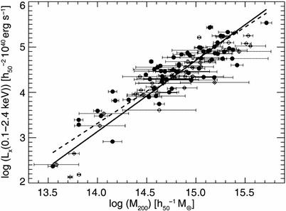
Fig. 6.44
For the galaxy clusters in the extended
HIFLUGCS sample, the X-ray luminosity in the energy range of the
ROSAT satellite is plotted versus the mass of the cluster. The
solid points show the clusters of the HIFLUGCS sample proper. For
the full sample and for the main HIFLUGCS sample, a best-fit power
law is indicated by the solid
line and dashed
line, respectively. Source: T. Reiprich & H. Böhringer
2002, The Mass Function of an
X-Ray Flux-limited Sample of Galaxy Clusters, ApJ 567, 716,
p. 726, Fig. 6. ©AAS. Reproduced with permission
This scaling relation can also be tested
empirically, as shown in Fig. 6.44, where the X-ray luminosity in the energy
range of the ROSAT satellite is plotted against the virial mass.
One can immediately see that clusters of galaxies indeed show a
strong correlation between luminosity and mass, but with a clearly
larger scatter than in the mass-temperature relation.9 Therefore, the temperature of the
intergalactic gas is a better mass indicator than the X-ray
luminosity or the velocity dispersion of the cluster
galaxies.
However, determining the slope of the relation
from the data approximately yields  , instead
of the expected behavior (
, instead
of the expected behavior ( ).
Obviously, the above scaling arguments are not valid with the
assumption of a constant gas fraction. This discrepancy between
theoretical expectations and observations has been found in several
samples of galaxy clusters and is considered well established. An
explanation is found in models where the intergalactic gas has been
heated not only by gravitational infall into the potential well of
the cluster. Other sources of heating may have been present or
still are. For cooler, less massive clusters, this additional
heating should have a larger effect than for the very massive ones,
which could also explain the deviation of low-M clusters from the mass-luminosity
relation of massive clusters visible in Fig. 6.44. As already argued
in the discussion of cooling flows in Sect. 6.4.3, an AGN in the
inner regions of the cluster may provide such a heating. The
kinetic energy provided by supernovae in cluster galaxies is also
considered a potential source of additional heating of the
intergalactic gas. Furthermore, the normalization of the
luminosity-mass relation appears to be significantly different for
cool-core clusters than for others, which supports the idea that
heating affects this relation. It is obvious that solving this
mystery will provide us with better insights into the formation and
evolution of the gas component in clusters of galaxies.
).
Obviously, the above scaling arguments are not valid with the
assumption of a constant gas fraction. This discrepancy between
theoretical expectations and observations has been found in several
samples of galaxy clusters and is considered well established. An
explanation is found in models where the intergalactic gas has been
heated not only by gravitational infall into the potential well of
the cluster. Other sources of heating may have been present or
still are. For cooler, less massive clusters, this additional
heating should have a larger effect than for the very massive ones,
which could also explain the deviation of low-M clusters from the mass-luminosity
relation of massive clusters visible in Fig. 6.44. As already argued
in the discussion of cooling flows in Sect. 6.4.3, an AGN in the
inner regions of the cluster may provide such a heating. The
kinetic energy provided by supernovae in cluster galaxies is also
considered a potential source of additional heating of the
intergalactic gas. Furthermore, the normalization of the
luminosity-mass relation appears to be significantly different for
cool-core clusters than for others, which supports the idea that
heating affects this relation. It is obvious that solving this
mystery will provide us with better insights into the formation and
evolution of the gas component in clusters of galaxies.
, instead
of the expected behavior ().
Obviously, the above scaling arguments are not valid with the
assumption of a constant gas fraction. This discrepancy between
theoretical expectations and observations has been found in several
samples of galaxy clusters and is considered well established. An
explanation is found in models where the intergalactic gas has been
heated not only by gravitational infall into the potential well of
the cluster. Other sources of heating may have been present or
still are. For cooler, less massive clusters, this additional
heating should have a larger effect than for the very massive ones,
which could also explain the deviation of low-M clusters from the mass-luminosity
relation of massive clusters visible in Fig. 6.44. As already argued
in the discussion of cooling flows in Sect. 6.4.3, an AGN in the
inner regions of the cluster may provide such a heating. The
kinetic energy provided by supernovae in cluster galaxies is also
considered a potential source of additional heating of the
intergalactic gas. Furthermore, the normalization of the
luminosity-mass relation appears to be significantly different for
cool-core clusters than for others, which supports the idea that
heating affects this relation. It is obvious that solving this
mystery will provide us with better insights into the formation and
evolution of the gas component in clusters of galaxies.Despite this discrepancy between the simple
models and the observations, Fig. 6.44 shows a clear
correlation between mass and luminosity, which can thus be used
empirically after having been calibrated. Although the temperature
is the preferred measure for a cluster’s mass, one will in many
cases resort to the relation between mass and X-ray luminosity
because determining the luminosity (in a fixed energy range) is
considerably simpler than measuring the temperature, for which
significantly better photon statistics, i.e., longer exposure times
are required.
6.5.4 The Y -parameter
The foregoing scaling relations connect the
cluster mass with an observable. We have seen that the relation
between cluster mass and gas temperature yields the smallest
dispersion; hence, the X-ray temperature provides the best mass
proxy of those that we considered above.
More recently, an alternative quantity for
estimating the cluster mass was introduced. We saw in
Sect. 6.4.4
above that the integrated SZ-effect is proportional to  , where is case of
non-isothermal temperature distribution T g needs to be interpreted
as density-weighted temperature. In analogy, one considers
, where is case of
non-isothermal temperature distribution T g needs to be interpreted
as density-weighted temperature. In analogy, one considers
 which is related to the thermal energy of gas in the cluster. The
gas mass is related to the total mass by
which is related to the thermal energy of gas in the cluster. The
gas mass is related to the total mass by  , where
f g is the
gas-mass fraction. Assuming this to be constant, and
using (6.52), we expect a scaling relation of the form
, where
f g is the
gas-mass fraction. Assuming this to be constant, and
using (6.52), we expect a scaling relation of the form
 Numerical simulations including hydrodynamics first suggested that
clusters should have a smaller scatter around the Y X-M relation than for the other scaling
relations. From X-ray observations, one indeed finds that clusters
obey a relation very close to (6.60), with a slightly
different slope, M ∝ Y 0. 55 (instead of 0.6).
Furthermore, the scatter around the Y X-M relation is smaller than that around
the T
X-M relation,
and in particular, at least for relaxed clusters, it is well
described by a power-law behavior. Hence, Y X provides a very useful
mass proxy.
Numerical simulations including hydrodynamics first suggested that
clusters should have a smaller scatter around the Y X-M relation than for the other scaling
relations. From X-ray observations, one indeed finds that clusters
obey a relation very close to (6.60), with a slightly
different slope, M ∝ Y 0. 55 (instead of 0.6).
Furthermore, the scatter around the Y X-M relation is smaller than that around
the T
X-M relation,
and in particular, at least for relaxed clusters, it is well
described by a power-law behavior. Hence, Y X provides a very useful
mass proxy.
, where is case of
non-isothermal temperature distribution T g needs to be interpreted
as density-weighted temperature. In analogy, one considers
(6.59)
, where
f g is the
gas-mass fraction. Assuming this to be constant, and
using (6.52), we expect a scaling relation of the form
(6.60)
Center-excised
scaling relations. We have seen that one can roughly divide
clusters into cool-core clusters, which show a strong peak in the
X-ray emission towards the center, and non-cool core clusters,
which are presumably dynamically disturbed. At first sight, one
would not expect that both types of clusters follow the same
scaling relations. Indeed, not only the temperature profile of
non-cool core clusters is different from that of cool-core
clusters, but as a consequence also their pressure profiles, which
is the relevant quantity for the SZ effect [see (6.47)]. Furthermore, we
have seen that feedback processes from a central AGN affect the
intracluster medium, causing (strong) deviations from spherical
symmetry and locally varying temperature. Hence, we would expect
that the central regions of clusters do not follow approximately
some ‘universal’ behavior or a corresponding scaling
relation.
However, if this central region is excised, the
shape of the pressure profiles of clusters closely follow a
universal profile, out to a radius of r 500 (see Fig. 6.45); for larger radii,
observations are difficult with the current X-ray observatories,
due to the high background and the fact that the X-ray surface
brightness decreases steeply for large radii. Hence, once the
central region is cut out in the analysis, clusters seem to form a
relatively homogeneous class of objects, despite all potential
complications of hydrodynamic effects. It is for this reason why
clusters can be used for cosmological studies, as we shall describe
in Sect. 8.2.
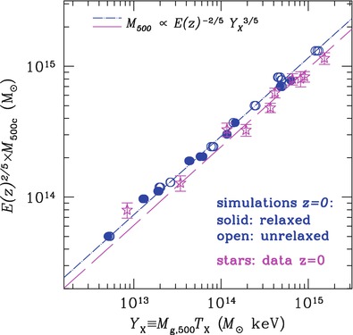
Fig. 6.45
The relation between the cluster mass
M 500 and the
Y X parameter.
For this figure, the central region of the clusters has been cut
out; specifically, the X-ray temperature was measured in the
annulus 0. 15r
500 ≤ r ≤ r 500. The blue points show results from simulated
clusters, where filled dots
correspond to relaxed (cool-core) clusters, open symbols to non-relaxed clusters.
It can be seen that both types of simulated clusters follow the
same power law between M
and Y X. A
sample of observed relaxed cluster is shown as star symbols; since these clusters are
not at redshift zero, as the simulated ones, a redshift correction
was applied to their masses (see Sect. 6.5.5 below). The
observed clusters follow a very similar power law, though with
a ∼ 15 % smaller normalization. Source: A.V. Kravtsov et al.
2006, A New Robust Low-Scatter
X-Ray Mass Indicator for Clusters of Galaxies, ApJ 650, 128,
p. 135, Fig. 7. ©AAS. Reproduced with permission
6.5.5 Redshift dependence of scaling relations
The foregoing relations between the quantities of
clusters were all obtained for very low-redshift objects. When
considering clusters at higher redshift, one might expect that
these scaling relations will evolve.
As mentioned before, the virial radius of a
cluster is defined by the mean density inside of it being larger
than the critical density by about a factor of Δ c ∼ 200. The critical
density is a function of redshift,  ,
where ρ cr,0 is
the critical density of the current universe [see (4.15)], and
,
where ρ cr,0 is
the critical density of the current universe [see (4.15)], and  . Since ρ cr is larger at higher
redshifts, the mean mass density inside clusters also increases,
. Since ρ cr is larger at higher
redshifts, the mean mass density inside clusters also increases,
 .
This affects also the scaling of the characteristic temperature of
the cluster,
.
This affects also the scaling of the characteristic temperature of
the cluster,
![$$\displaystyle{ T\propto \frac{M_{\mathrm{vir}}} {r_{\mathrm{vir}}} = M_{\mathrm{vir}}^{2/3}\!\left (\frac{M_{\mathrm{vir}}} {r_{\mathrm{vir}}^{3}} \right )^{1/3}\!\propto M_{\mathrm{ vir}}^{2/3}\left \langle \rho \right \rangle ^{1/3}\propto \left [M_{\mathrm{ vir}}E(z)\right ]^{2/3}. }$$](A129044_2_En_6_Chapter_Equ61.gif)
,
where ρ cr,0 is
the critical density of the current universe [see (4.15)], and . Since ρ cr is larger at higher
redshifts, the mean mass density inside clusters also increases,
.
This affects also the scaling of the characteristic temperature of
the cluster,
(6.61)
The bolometric X-ray luminosity, assumed to be
due to bremsstrahlung only, is the volume integral over the
emissivity (6.32), and so scales like
 where we assumed a constant temperature of the intracluster gas. If
the gas fraction of clusters is a constant, i.e., independent of
mass and redshift, then we expect
where we assumed a constant temperature of the intracluster gas. If
the gas fraction of clusters is a constant, i.e., independent of
mass and redshift, then we expect  ,
assuming the clumping factor
,
assuming the clumping factor  to stay constant. Together with (6.61), we then obtain the
expected scaling of the luminosity,
to stay constant. Together with (6.61), we then obtain the
expected scaling of the luminosity,
![$$\displaystyle{ \frac{L_{\mathrm{bol}}} {E(z)} \propto \left [M_{\mathrm{vir}}\,E(z)\right ]^{4/3}\;. }$$](A129044_2_En_6_Chapter_Equ62.gif) Finally, for the Y
-parameter, we have
Finally, for the Y
-parameter, we have ![$$Y = M_{\mathrm{gas}}\,T \propto M_{\mathrm{vir}}\,\left [M_{\mathrm{vir}}\,E(z)\right ]^{2/3}$$](A129044_2_En_6_Chapter_IEq80.gif) ,
where we again assumed a constant gas fraction and
used (6.61); thus,
,
where we again assumed a constant gas fraction and
used (6.61); thus,
![$$\displaystyle{ Y \,E(z) \propto \left [M_{\mathrm{vir}}\,E(z)\right ]^{5/3}\;. }$$](A129044_2_En_6_Chapter_Equ63.gif) These relation generalize (6.52), (6.57) and (6.60) to higher redshifts
(note that this redshift dependence was included in
Fig. 6.45).
If we assume that the profiles of clusters are self-similar, i.e.,
their density and temperature profiles all have the same shape, but
different amplitude and scale length, then these relation do not
only apply to the virial radius, but also for regions with
different density thresholds.
These relation generalize (6.52), (6.57) and (6.60) to higher redshifts
(note that this redshift dependence was included in
Fig. 6.45).
If we assume that the profiles of clusters are self-similar, i.e.,
their density and temperature profiles all have the same shape, but
different amplitude and scale length, then these relation do not
only apply to the virial radius, but also for regions with
different density thresholds.
,
assuming the clumping factor
to stay constant. Together with (6.61), we then obtain the
expected scaling of the luminosity,
(6.62)
,
where we again assumed a constant gas fraction and
used (6.61); thus,
(6.63)

Fig. 6.46
The cluster mass-X-ray luminosity relation,
where the mass was determined with weak gravitational lensing
methods. Dark blue diamonds
and sienna crosses indicate
mass measurements of individual clusters. This is feasible only for
high-mass objects. The other data points indicate mean masses of
sets of clusters within given L-bins. In particular, the red squares were obtained from a weak
lensing analysis of X-ray clusters in the COSMOS field, for which
the three highest redshift bins are explicitly indicated. The
shaded region indicates the
range which power-law fits within the 1-σ range to the data would cover.
Source: A. Leauthaud et al. 2010, A Weak Lensing Study of X-ray Groups in the
Cosmos Survey: Form and Evolution of the Mass-Luminosity
Relation, ApJ 709, 97, p. 109, Fig. 6. ©AAS. Reproduced
with permission
In detail, these scaling relations are observed
to be somewhat different. Whereas the redshift scaling in the
mass-temperature relation (6.61) seems to apply to high-redshift clusters,
the redshift scaling in the mass-luminosity
relation (6.62) is not supported by observations;
instead, the redshift evolution is observed to be slower than
predicted by the self-similar model. Finally, Fig. 6.46 shows the
mass-luminosity relation, where the mass determination was done via
weak lensing analysis. Whereas there is a very tight correlation
between luminosity and mass, the slope of the best-fitting power
law is flatter than predicted by the self-similar
behavior (6.62), which probably indicates that clusters
are not truly self-similar.
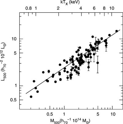
Fig. 6.47
The correlation between K-band luminosity
and the mass of galaxy clusters, measured within the radius inside
of which the mean density is 500 times the critical density of the
Universe. The cluster mass was determined by the
relation (6.53) between mass and temperature. Source:
Y.-T. Lin et al. 2004, K-Band
Properties of Galaxy Clusters and Groups: Luminosity Function,
Radial Distribution, and Halo Occupation Number, ApJ 610,
745, p. 753, Fig. 3. ©AAS. Reproduced with permission
6.5.6 Near-infrared luminosity as mass indicator
Whereas the optical luminosity of galaxies
depends not only on the mass of the stars but also on the star
formation history, the NIR light is much less dependent on the
latter. As we have discussed before, the NIR luminosity is thus
quite a reliable measure of the total mass in stars. For this
reason, we would expect that the NIR luminosity of a cluster is
tightly correlated with its total stellar mass. Furthermore, if the
latter is closely related to the total cluster mass, as would be
the case if the stellar mass is a fixed fraction of the cluster’s
total mass, the NIR luminosity can be used to estimate the masses
of clusters.
The Two Micron All Sky Survey (2MASS) provides
the first opportunity to perform such an analysis on a large sample
of galaxy clusters. One selects clusters of galaxies for which
masses were determined by X-ray methods, and then measures the
K-band luminosities of the galaxies within the cluster.
Figure 6.47 presents the resulting mass-luminosity
diagram within r
500 for 93 galaxy clusters and groups, where the mass
was derived from the clusters’ X-ray temperatures (plotted on the
top axis) by means of (6.53). A surprisingly close relation between
these two parameters is seen, which can be described by a power law
of the form
 where a Hubble constant of h = 0. 7 is assumed. The dispersion of
individual clusters around this power law is about 32 %, where at
least part of this scatter originates in uncertainties in the mass
determination—thus, the intrinsic scatter is even smaller. This
result is of great potential importance for future studies of
galaxy clusters, and it renders the NIR luminosity a competitive
method for the determination of cluster masses, which is of
considerable interest in view of the current and future generation
of NIR wide-field instruments (like VISTA on Paranal, for
instance).
where a Hubble constant of h = 0. 7 is assumed. The dispersion of
individual clusters around this power law is about 32 %, where at
least part of this scatter originates in uncertainties in the mass
determination—thus, the intrinsic scatter is even smaller. This
result is of great potential importance for future studies of
galaxy clusters, and it renders the NIR luminosity a competitive
method for the determination of cluster masses, which is of
considerable interest in view of the current and future generation
of NIR wide-field instruments (like VISTA on Paranal, for
instance).
(6.64)
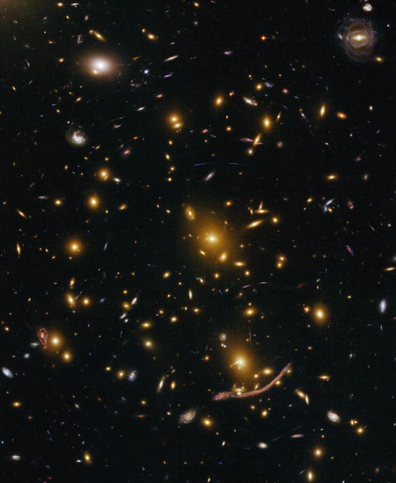
Fig. 6.48
The cluster of galaxies A 370 at redshift
z = 0. 375 is one of the
first two clusters in which giant luminous arcs were found in 1986.
In this HST image, the arc is clearly visible; it is about 20
′ ′ long,
tangentially oriented with respect to the center of the cluster
which is located roughly halfway between the two brightest cluster
galaxies, and curved towards the center of the cluster. The arc is
the image of a galaxy at z
s = 0. 724. Several other very thin arcs are clearly
seen, many of which appear in close pairs; in these cases, they are
multiple images of the same source galaxy. Only with HST images was
it realized how thin these arcs are. One also notes the presence of
a ‘radial arc’, not far from the bright galaxy closest to the major
arc. Credit: NASA, ESA, the Hubble SM4 ERO Team, and ST-ECF
6.6 Clusters of galaxies as gravitational lenses
6.6.1 Luminous arcs
In 1986, two groups independently discovered
unusually stretched, arc-shaped sources in two clusters of galaxies
at high redshift (see Figs. 6.48 and 6.49). The nature of
these sources was unknown at first; they were named arcs, or giant luminous arcs, which did not
imply any interpretation originally. Different hypotheses for the
origin of these arcs were formulated, like for instance emission by
shock fronts in the ICM, originating from explosive events. All
these scenarios were disproven when the spectroscopy of the arc in
the cluster Abell 370 showed that the source is at a much higher
redshift than the cluster itself. Thus, the arc is a background
source, subject to the gravitational lens effect (see
Sect. 3.11) of the cluster. By
differential light deflection, the light beam of the source can be
distorted in such a way that highly elongated arc-shaped images are
produced.
The discovery that clusters of galaxies may act
as strong gravitational lenses came as a surprise at that time.
Based on the knowledge about the mass distribution of clusters,
derived from X-ray observations before ROSAT, it was estimated that
the central surface mass density of clusters is not sufficiently
high for strong effects of gravitational light deflection to occur.
This incorrect estimate of the central surface mass density in
clusters originated from analyses utilizing the β-model which, as briefly discussed
above, starts with some heavily simplifying assumptions.10
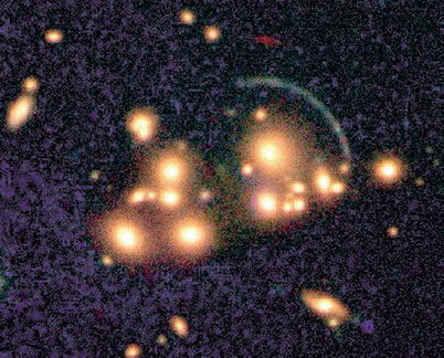
Fig. 6.49
The cluster of galaxies Cl 2244−02 at
redshift z = 0. 33 is the
second cluster in which an arc was discovered. Spectroscopic
analysis of this arc revealed the redshift of the corresponding
source to be z
s = 2. 24—at the time of discovery in 1987, it was the
first normal galaxy detected at a redshift > 2. This image was
observed with the near-IR camera ISAAC at the VLT. Above the arc,
one can see another strongly elongated red source which is probably
associated with a galaxy at very high redshift as well. Credit:
European Southern Observatory
Hence, arcs are strongly distorted and highly
magnified images of galaxies at high redshift. In some massive
clusters several arcs were discovered and the unique angular
resolution of the HST played a crucial role in such observations.
Some of these arcs are so thin that their width is unresolved even
by the HST, indicating an extreme length-to-width ratio. For many
arcs, additional images of the same source were discovered,
sometimes called ‘counter arcs’. The identification of multiple
images is performed either by optical spectroscopy (which is
difficult in general, because one arc is highly magnified while the
other images of the same source are considerably less strongly
magnified and therefore much fainter in general, together with the
fact that spectroscopy of faint sources is very time-consuming), by
multi-color photometry (all images of the same source should have
the same color), or by common morphological properties.
Lens
models. Once again, the simplest mass model for a galaxy
cluster as a lens is the singular isothermal sphere (SIS). This
lens model was discussed previously in Sect. 3.11.2. Its characteristic angular
scale is specified by the Einstein radius (3.75), or
 Very high magnifications and distortions of images can occur only
very close to the Einstein radius. This immediately yields an
initial mass estimate of a cluster, by assuming that the Einstein
radius is about the same as the angular separation of the arc from
the center of the cluster. The projected mass within the Einstein
radius can then be derived, using (3.81). Since clusters of galaxies
are, in general, not spherically symmetric and may show significant
substructure, so that the separation of the arc from the cluster
center may deviate significantly from the Einstein radius, this
mass estimate is not very accurate in general; the uncertainty is
presumably ∼ 30 %. Models with asymmetric mass distributions
predict a variety of possible morphologies for the arcs and the
positions of multiple images, as is demonstrated in
Fig. 6.50 for
an elliptical lens. If several arcs are discovered in a cluster, or
several images of the source of an arc, we can investigate detailed
mass models for such a cluster. The accuracy of these models
depends on the number and positions of the observed lensed images;
e.g., on how many arcs and how many multiple image systems are
available for modeling. The resulting mass models are not
unambiguous, but they are robust. Clusters that contain many lensed
images have very well-determined mass properties, for instance the
mass and the mass profile within the radii at which arcs are found,
or the ellipticity of the mass distribution and its
substructure.
Very high magnifications and distortions of images can occur only
very close to the Einstein radius. This immediately yields an
initial mass estimate of a cluster, by assuming that the Einstein
radius is about the same as the angular separation of the arc from
the center of the cluster. The projected mass within the Einstein
radius can then be derived, using (3.81). Since clusters of galaxies
are, in general, not spherically symmetric and may show significant
substructure, so that the separation of the arc from the cluster
center may deviate significantly from the Einstein radius, this
mass estimate is not very accurate in general; the uncertainty is
presumably ∼ 30 %. Models with asymmetric mass distributions
predict a variety of possible morphologies for the arcs and the
positions of multiple images, as is demonstrated in
Fig. 6.50 for
an elliptical lens. If several arcs are discovered in a cluster, or
several images of the source of an arc, we can investigate detailed
mass models for such a cluster. The accuracy of these models
depends on the number and positions of the observed lensed images;
e.g., on how many arcs and how many multiple image systems are
available for modeling. The resulting mass models are not
unambiguous, but they are robust. Clusters that contain many lensed
images have very well-determined mass properties, for instance the
mass and the mass profile within the radii at which arcs are found,
or the ellipticity of the mass distribution and its
substructure.
(6.65)
Figure 6.51 shows two clusters of galaxies which
contain several arcs. The lensing mass estimate of the cluster
Cl 0024+17 is quite different from the mass obtained through an
X-ray analysis. Spectroscopy of its member galaxies show evidence
for a bimodal distribution in velocity space which is interpreted
as the cluster being indeed a pair of clusters, colliding along the
line-of-sight. If this interpretation is correct, the mass estimate
from X-rays is expected to yield discordant values.
For a long time, A 2218 was the classic example
of the existence of numerous arcs in a single galaxy cluster. Then
after the installation of the ACS camera on-board HST in 2002, a
spectacular image of the cluster A 1689 was obtained in which more
than 100 arcs and multiple images were identified (see
Fig. 6.52).
Several zoomed sections of this image are shown in the lower part
of the figure. For clusters of galaxies with such a rich inventory
of lens phenomena, very detailed mass models can be
constructed.
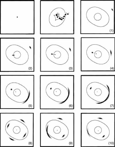
Fig. 6.50
Distortions by the lens effect of an
elliptical potential, as a function of the source position. The
first panel shows the
source itself. The second
panel displays ten positions of the source in the source
plane (numbered from 1 to 10) relative to the center of the lens;
the solid curves show the
inner and outer caustics. The remaining panels (numbered from 1 to
10) show the inner and outer critical curves and the resulting
images of the source. Source: B. Fort & Y. Mellier 1994,
Arc(let)s in clusters of
galaxies, A&AR 5, 239. © Springer-Verlag. Reproduced
with permission
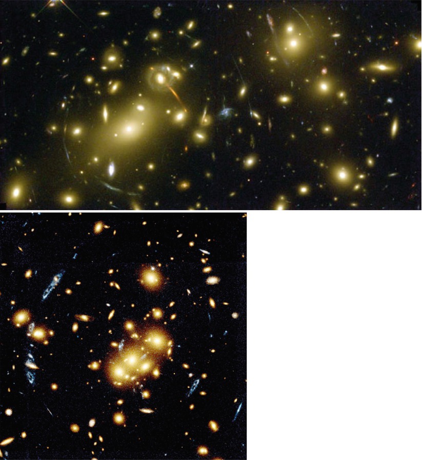
Fig. 6.51
Top: the cluster of galaxies A 2218
(z d = 0. 175)
contains one of the most spectacular arc systems. The majority of
the galaxies visible in the image are associated with the cluster,
and the redshifts of many of the strongly distorted arcs have now
been measured. Bottom: the
cluster of galaxies Cl 0024+17 (z d = 0. 39) contains a rich
system of arcs. The arcs appear bluish, stretched in a direction
which is tangential to the cluster center. The three arcs to the
left of the cluster center, and the arc to the right of it and
closer to the center, are images of the same background galaxy
which has a redshift of z
s = 1. 62. Another image of the same source was found
close to the cluster center. Also note the identical
(‘pretzel’-shaped) morphology of the images. Credit: Top: W. Couch/University of New South
Wales, R.S. Ellis/Cambridge University and NASA. Bottom: W.N. Colley and E.
Turner/Princeton University, J.A. Tyson/Bell Labs, Lucent
Technologies, and NASA
Fig. 6.52
The cluster of galaxies Abell 1689 has one
of the richest system of arcs and multiple images found to date. In
a deep ACS exposure of this cluster, shown on top with the X-ray emission
superimposed in blue, more
than a hundred such lensed images were detected. Six zoomed
sections of this ACS image are shown in the bottom part, in which various arcs are
visible, some with an extreme length-to-width ratio, indicating
very high magnification factors. Credit: X-ray: NASA/CXC/MIT/E.-H.
Peng et al.; optical: NASA, N. Benitez/JHU, T.
Broadhurst/Racah Institute of Physics/The Hebrew University, H.
Ford/JHU, M. Clampin/STScI, G. Hartig/STScI, G.
Illingworth/UCO/Lick Observatory, the ACS Science Team and
ESA
Such mass models have predictive power, allowing
an iterative modeling process. An initial simple mass model is
fitted to the most prominent lensed images in the observation,
i.e., either giant arcs or clearly recognizable multiple images. In
general, this model then predicts further images of the source
producing the arc. Close to these predicted positions, these
additional images are then searched for, utilizing the morphology
of the light distribution and the color. If this initial model
describes the overall mass distribution quite well, such images are
found. The exact positions of the new images provide further
constraints on the lens model which is then refined accordingly.
Again, the new model will predict further multiple image systems,
and so on. By this procedure, very detailed models can sometimes be
obtained. Since the lens properties of a cluster depend on the
distance or the redshift of the source, the redshift of lensed
sources can be predicted from the identification of multiple image
systems in clusters if a detailed mass model is available. These
predictions can then be verified by spectroscopic analysis, and the
success of this method gives us confidence in the accuracy of the
lens models.
Results. We
can summarize the most important results of the examination of
clusters using arcs and multiple images as follows: the mass of
galaxy clusters is indeed much larger than the mass of their
luminous matter. The lensing method yields a mass which is in very
good agreement with mass estimates from the X-ray method or from
dynamical methods. However, the core radius of clusters, i.e., the
scale on which the mass profile flattens inwards, is significantly
smaller than determined from X-ray observations. If the mass
distribution in clusters has a core, its size is estimated to be
r
c ∼ 30h
−1 kpc, in contrast to ∼ 150h −1 kpc obtained from early
X-ray analyses.11
This difference leads to a discrepancy in the mass determination
between the two methods on scales below ∼ 200h −1 kpc.
We emphasize that, at least in principle, the
mass determination based on arcs and multiple images is
substantially more accurate because it does not require any
assumptions about the symmetry of the mass distribution, about
hydrostatic equilibrium of the X-ray gas, or about an isothermal
temperature distribution. On the other hand, the lens effect
measures the mass in cylinders because the lens equation contains
only the projected mass distribution, whereas the X-ray method
determines the mass inside spheres. The conversion between the two
methods introduces uncertainties, in particular for clusters which
deviate significantly from spherical symmetry. Overestimating the
core radius was the main reason why the discovery of the arcs was a
surprise because clusters with core radii like the ones determined
from the early X-ray measurements would in fact not act as strong
gravitational lenses. Hence, the mere existence of arcs shows that
the core radius must be small.
A closer analysis of galaxy clusters with a cool
core shows that, in these clusters, the mass profile estimated from
X-ray observations is compatible with the observed arcs. Such
clusters are considered dynamically relaxed, so that for them the
assumption of a hydrostatic equilibrium is well justified. The
X-ray analysis has to account explicitly for the existence of an
inner cool region, though, and the accordingly modified X-ray
emission profile is more sophisticated than the simple β-model. Clusters without a cool core
are distinctly more complex dynamically. Besides the discrepancy in
mass determination, lensing and X-ray methods can lead to different
estimates of the center of mass in such unrelaxed clusters, which
may indicate that the gas has not had enough time since the last
strong interaction or merging process to settle into an equilibrium
state.
As we mentioned before, the cluster Cl 0024+17 in
Fig. 6.51
most likely has a complex structure along the line-of-sight, and
hence it is not surprising that X-ray estimated masses deviate
significantly from those obtained by lensing. As a second example,
the cluster A 1689 (Fig. 6.52) presumably also has a complex structure.
A combined lensing, X-ray and SZ-study of this cluster suggests
that it is highly elongated, with an axis ratio of ∼ 2 and the long
axis close to the line of sight. This orientation maximizes the
lensing strength of a triaxial mass distribution, and clusters
selected by their strong lensing features will be biased towards
these orientations. In order to account for the differences in mass
estimates from these different methods, one concludes that the gas
is not in hydrostatic equilibrium, but there must be substantial
fraction of non-thermal pressure in that cluster, e.g., from
turbulent motions of the intracluster gas.
The mass distribution in clusters often shows
significant substructure. Many clusters of galaxies in which arcs
are observed are not relaxed. These clusters still undergo
dynamical evolution—they are young systems with an age not much
larger than t
cross, or systems whose equilibrium was disturbed by a
fairly recent merger process. For such clusters, the X-ray method
is not well founded because the assumptions about symmetry and
equilibrium are not satisfied. The distribution of arcs in the
cluster A2218 (Fig. 6.51) clearly indicates a non-spherical mass
distribution. Indeed, this cluster seems to consist of at least two
massive components around which the arcs are curved, indicating
that the cluster is currently undergoing a strong merging event.
This is further supported by measurements of the temperature
distribution of the intracluster gas, which shows a strong peak in
the center, where the temperature is about a factor of two higher
than in its surrounding region.
From lens models, we find that for clusters with
a central cD galaxy, the orientation of the mass distribution
follows that of the cD galaxy quite closely. We conclude from this
result that the evolution of the brightest cluster galaxy must be
closely linked to the evolution of the cluster, e.g., by accretion
of a cooling flow onto the BCG or due to mergers with other cluster
members. Often, the shape of the mass distribution very well
resembles the galaxy distribution and the X-ray emission.
The investigation of galaxy
clusters with the gravitational lens method provides a third,
completely independent method of determining cluster masses. It
confirms that the mass of galaxy clusters significantly exceeds
that of the visible matter in stars and in the intracluster gas. We
conclude from this result that clusters of galaxies are dominated
by dark matter.
6.6.2 The weak gravitational lens effect
The principle of
the weak lensing effect. In Sect. 3.11 we saw that gravitational light
deflection does not only deflect light beams as a whole, but also
that the size and shape of light beams are distorted by
differential light deflection. This differential light deflection
leads, e.g., to sources appearing brighter than they would be
without the lens effect. The giant arcs discussed above are a very
clear example of these distortions and the corresponding
magnifications.
If some background sources exist which are
distorted in such an extreme way as to appear as giant luminous
arcs, then it is plausible that many more background galaxies
should exist which are less strongly distorted. Typically, these
are located at larger angular separations from the cluster center,
where the lens effect is weaker than at the locations of the
luminous arcs. Their distortion then is so weak that it cannot be
identified in an individual galaxy image. The reason for this is
that the intrinsic light distribution of galaxies is not circular;
rather, the observed image shape is a superposition of the
intrinsic shape and the gravitational lens distortion. The former
is considerably larger than the latter, in general, and acts as a
kind of noise in the measurement of the lensing effect. However,
the distortion of adjacent galaxy images should be similar since
the gravitational field their light beams are traversing is
similar. By averaging over many such galaxy images, the distortion
can then be measured (see Fig. 6.53) because no preferred direction exists in
the intrinsic orientation of galaxies; it is expected to be random.
After the results from the Hubble Deep Field (Fig. 1.37) became available, if not
before, we have known that the sky is densely covered by small,
faint galaxies. In deep optical images, one therefore finds a high
number density of such galaxies located in the background of a
galaxy cluster. Their measured shapes can be used for investigating
the weak lensing effect of the cluster.
Fig. 6.53
The principle of the weak gravitational
lensing effect is illustrated here with a simulation. Due to the
tidal component of the gravitational field in a cluster, the shape
of the images (ellipses) of background galaxies get distorted and,
as for arcs, the galaxy images will be aligned, on average,
tangentially to the cluster center. By local averaging over the
ellipticities of galaxy images, a local estimate of the tidal
gravitational field can be obtained (the direction of the sticks
indicates the orientation of the tidal field, and their length is
proportional to its strength). From this estimated tidal field, the
projected mass distribution can then be reconstructed. Source: C.
Seitz, The determination of the
mass distribution in clusters of galaxies by gravitationally
distorted images of background galaxies, Dissertation, LMU
München, 1996
Fig. 6.54
On the
left, the tidal (or shear) field of the cluster Cl 0024+17
(Fig. 6.51)
is indicated by sticks whose length and direction represent the
strength and orientation of the tidal gravitational field.
On the right, the surface
mass density is shown, reconstructed by means of the weak
gravitational lens effect. The bright galaxies in the cluster are
seen to follow the (dark) matter distribution; the orientation of
the isodensity contours is the same as the orientation of the light
in the center of the cluster. Credit: optical image: HST/NASA,
Colley et al.; shear field and mass reconstruction: C. Seitz,
The determination of the mass
distribution in clusters of galaxies by gravitationally distorted
images of background galaxies, Dissertation, LMU München,
1996
The distortion, obtained by averaging over image
ellipticities, reflects the contribution of the tidal forces to the
local gravitational field of the cluster. In this context, it is
denoted as shear. It is
given by the projection of the tidal component of the gravitational
field along the line-of-sight. The shear results from the
derivative of the deflection angle, where the deflection
angle (3.62) depends linearly on the
surface mass density of the lens. Hence, it is possible to
reconstruct the surface mass density of galaxy clusters in a
completely parameter-free way using the measured shear: it can be
used to map the (total, i.e., dark plus luminous) matter in a
cluster.
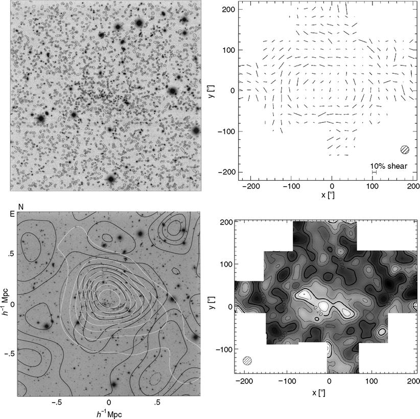
Fig. 6.55
Analysis of the cluster of galaxies
MS 1054−03 by the weak lensing effect. In the upper left panel, a ground-based image
is shown with a field size of 7.′5 ×
7.′5. In this image, about 2400 faint objects are
detected, the majority of which are galaxies at high redshift. From
the measured ellipticities of the galaxies, the tidal field of the
cluster can be reconstructed, and from this the projected mass
distribution  , presented in the
lower left panel; the
latter is indicated by the black contours, while the white contours
represent the smoothed light distribution of the cluster galaxies.
A mosaic of HST images allows the ellipticity measurement of a
significantly larger number of galaxies, and with better accuracy.
The tidal field resulting from these measurements is displayed in
the upper right panel, with
the reconstructed surface mass density shown in the lower right panel. One can clearly see
that the cluster is strongly structured, with three density maxima
which correspond to regions with bright cluster galaxies. This
cluster seems to be currently in the process of formation through a
merger of smaller entities. Source: Left: G.A. Luppino & N. Kaiser
1997, Detection of Weak Lensing by
a Cluster of Galaxies at z = 0.83, ApJ 475, 20, PLATE 2, 3,
Figs. 3, 5. ©AAS. Reproduced with permission. Right: H. Hoekstra et al. 2000,
Hubble Space Telescope
Weak-Lensing Study of the z = 0.83 Cluster MS 1054–03, ApJ
532, 88, p. 94, 96, Figs. 9, 12. ©AAS. Reproduced with
permission
, presented in the
lower left panel; the
latter is indicated by the black contours, while the white contours
represent the smoothed light distribution of the cluster galaxies.
A mosaic of HST images allows the ellipticity measurement of a
significantly larger number of galaxies, and with better accuracy.
The tidal field resulting from these measurements is displayed in
the upper right panel, with
the reconstructed surface mass density shown in the lower right panel. One can clearly see
that the cluster is strongly structured, with three density maxima
which correspond to regions with bright cluster galaxies. This
cluster seems to be currently in the process of formation through a
merger of smaller entities. Source: Left: G.A. Luppino & N. Kaiser
1997, Detection of Weak Lensing by
a Cluster of Galaxies at z = 0.83, ApJ 475, 20, PLATE 2, 3,
Figs. 3, 5. ©AAS. Reproduced with permission. Right: H. Hoekstra et al. 2000,
Hubble Space Telescope
Weak-Lensing Study of the z = 0.83 Cluster MS 1054–03, ApJ
532, 88, p. 94, 96, Figs. 9, 12. ©AAS. Reproduced with
permissionObservations. Since shear measurements
are based on averaging over image ellipticities of distant
galaxies, this method of weak
gravitational lensing requires optical images with as high a
galaxy density as possible. This implies that the exposures need to
be very deep to reach very faint magnitudes. But since very faint
galaxies are also very distant and, as a consequence, have small
angular extent, the observations need to be carried out under very
good observing conditions, to be able to accurately measure the
shape of galaxy images without them being smeared into circular
images by atmospheric turbulence, i.e., the seeing. Typically, to
apply this method images from 4-m class telescopes are used, with
exposure times of 1–3 h. This way, we reach a density of about 30
galaxies per square arcminute (thus, 105 per square
degree) of which shapes are sufficiently well measurable. This
corresponds to a limiting magnitude of about R ∼ 25. The seeing during the exposure
should not be larger than ∼ 0.″8 to still be able to
correct for effects of the point-spread function. The smaller the
seeing, the more galaxy images can be used for the weak lensing
analysis.
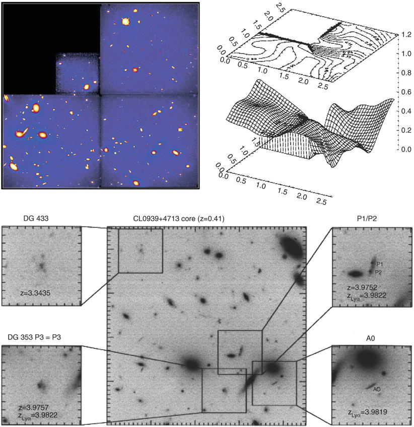
Fig. 6.56
The cluster of galaxies Cl 0939+4713 (A851)
is the cluster with the highest redshift in the Abell catalog. The
HST image in the upper left
panel was obtained shortly after the refurbishment of the
HST in 1994; in this image, North is down, whereas it is up in the
bottom images. The mass
distribution of the cluster was reconstructed from this image and
is shown in the upper right
panel, both as the level surface and by the contours on top.
We see that the distributions of bright galaxies and of (dark)
matter are very similar: their respective centers are aligned, a
secondary maximum exists in both the light and the matter
distribution, as does the prominent minimum in which no bright
galaxies are visible either. A higher-resolution mass map from the
weak lensing data predicts that the cluster is critical near its
center, i.e., able to produce strong lensing features. Indeed,
these were observed, as can be seen from the image at the
bottom: a triple image
system at z ≈ 3. 98 and an
arc with z = 3. 98 were
confirmed spectroscopically. Source: Top: C. Seitz et al. 1996,
The mass distribution of
CL0939+4713 obtained from a ‘weak’ lensing analysis of a WFPC2
image., A&A 314, 707, p. 708, 712, Figs. 1, 5.
©ESO. Reproduced with permission. Bottom: S.C. Trager et al. 1997,
Galaxies at z ≈ 4 and the
Formation of Population II, ApJ 485, 92, p. 93, Fig. 1.
©AAS. Reproduced with permission
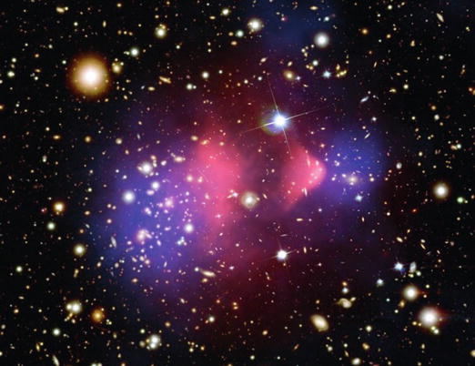
Fig. 6.57
The Bullet cluster, shown before in
Fig. 6.34. In
red, the X-ray emission is
shown, superposed on the HST image of the cluster. In blue, the weak lensing mass
reconstruction is shown, which is located on the galaxy
concentrations of the two colliding clusters. Credit: X-ray:
NASA/CXC/CfA/M. Markevitch et al.; Optical: NASA/STScI;
Magellan/U. Arizona/D. Clowe et al.; Lensing Map: NASA/STScI;
ESO WFI; Magellan/U.Arizona/D. Clowe et al.
Systematic observations of the weak lensing
effect only became feasible with the development of wide-field
cameras.12 This,
together with the improvement of the dome seeing at many telescopes
and the development of dedicated software for data analysis,
rendered quantitative observational studies with weak lensing
possible; the best telescopes at the best observatories regularly
accomplish seeing below 0.″8, and the dedicated
software is specifically designed for measuring the shapes of
extremely faint galaxy images and for correcting for the effects of
seeing and anisotropy of the point spread function.
Mass
reconstruction of galaxy clusters. By means of this method,
the reconstruction of the mass density of a large number of
clusters became possible. The most important results of these
investigations are as follows: the center of the mass distribution
corresponds to the optical center of the cluster (see
Fig. 6.54).
If X-ray information is available, the mass distribution is, in
general, found to be centered on the X-ray maximum, except in
clusters which are heavily disturbed. The shape of the mass
distribution—e.g., its ellipticity and orientation—is in most cases
very similar to the distribution of bright cluster galaxies. The
comparison of the mass profile determined by this method and that
determined from X-ray data agree well, typically within a factor
of ∼ 1. 5; we will discuss mass profiles of clusters from weak
lensing further below (Sect. 7.7) where we compare them with
cosmological predictions.
Through the weak lensing effect, substructure in
the mass distribution is also detected in some clusters
(Fig. 6.55)
which does not in all cases reflect the distribution of cluster
galaxies. However, in general a good correspondence between light
and mass exists (Fig. 6.56). From these lensing studies, we obtain a
mass-to-light ratio for clusters that agrees with that found from
X-ray analyses, about M∕L ∼ 250h in Solar units. Clusters of galaxies
that strongly deviate from this average value do exist, however.
Two independent analyses for the cluster MS 1224+20 resulted in a
mass-to-light-ratio of M∕L ≈ 800h in Solar units, more than twice the
value normally found in clusters.
The similarity of the mass and galaxy
distributions is not necessarily expected because the lens effect
measures the total mass distribution, and therefore mainly the dark
matter in a cluster of galaxies. The similar distributions then
imply that the galaxies in a cluster seem to basically follow the
distribution of the dark matter (Sect. 7.6.1), although there are some
exceptions.
Bullet clusters,
and the nature of dark matter. Figure 6.34 shows the X-ray
emission and the galaxy distribution of the so-called Bullet
cluster, actually a system of two clusters which have recently
collided. Besides the hydrodynamic effects of the collision, this
system is of great interest to test for the nature of the
discrepancy between the observed mass in clusters (from the stars
in the member galaxies and the intracluster gas) and the
gravitational mass deduced from the X-ray emission, the galaxy
peculiar velocities in clusters, and the lensing results. If this
discrepancy is due to a modification of the law of gravity on large
scales, as was speculated, then we expect that the bulk of the mass
in the Bullet cluster is centered on the X-ray emitting gas, since
its mass is several times higher than that of the stars in the
cluster galaxies. On the other hand, if the discrepancy is due to
(collisionless) dark matter, then this dark matter should behave
similarly to the galaxies in a collision: the scattering cross
section is very small, and thus the dark matter components of both
colliding clusters (like the galaxies) just run through each other.
So: where’s the mass?
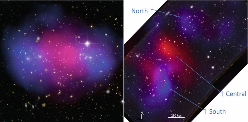
Fig. 6.58
Two clusters which are similar to the
Bullet cluster. Left panel:
The cluster MACS J0025.4−1222 has undergone a recent collision
between two separate clusters. The two galaxy concentrations are
seen at the left and right side of the optical image, which was
taken with the HST. Shown in pink is the X-ray emission from this
cluster, observed with Chandra. Using the weak lensing technique,
the mass distribution of this cluster was reconstructed and is
shown in blue. As for the
Bullet cluster, the total mass distribution traces that of the
galaxies, and is very different from the distribution of the hot
intracluster gas. Right
panel: The merging cluster DLSCL J0916.2+2951 at
z = 0. 53 also has its hot
gas (indicated by the X-ray emission shown in red) displaced from the two
concentrations of cluster galaxies, denoted by ‘North’ and ‘South’
in the image. In blue, the
weak lensing mass reconstruction of this cluster is shown, again
centered on the galaxy concentrations and clearly displaced from
the intracluster gas. Credit: Left: NASA, ESA, CXC, M. Bradac
(University of California, Santa Barbara), and S. Allen (Stanford
University). Right: W.D.
Dawson et al. 2012, Discovery
of a Dissociative Galaxy Cluster Merger with Large Physical
Separation, ApJ 747, L42, p. 2, Fig. 1. ©AAS.
Reproduced with permission
This question can be answered unambiguously with
the weak lensing effect; the result is displayed in
Fig. 6.57.
The mass is centered on the galaxy distributions of the two
clusters, and clearly displaced from the X-ray emitting gas.
Therefore, the mass discrepancy cannot be ascribed to a
modification of the law of gravity; instead, the main mass
component of the clusters must behave very similarly as the
galaxies, i.e., collisionless. Thus, the Bullet cluster provides
the clearest direct proof for the existence of dark matter. Whereas
the Bullet cluster was the first of its kind, in the meantime other
cluster collisions have been investigated as well. Two other
clusters with very similar behavior are shown in Fig. 6.58.
The weak lensing results from
clusters in collision cannot be explained without the existence of
collisionless dark matter in galaxy clusters, even if modifications
of the law of gravity on large scales were allowed for.
Dark matter
filaments between cluster pairs. The hierarchical structure
growth in the Universe, a consequence of the Cold Dark Matter
model, predicts that mass concentrations form near the intersection
points of dark matter filaments, through which they accrete mass
(see Chap. 7). These filaments in general have a
density too low to produce a detectable weak lensing signal.
However, if two large mass concentrations, such as two clusters,
are relatively close to each other, the density of the filament
between them is expected to be considerably higher than in the
mean. Therefore, pairs of galaxy clusters are the best locations to
look for dark matter filaments that connect the members of the
pair. Indeed, several attempts for the detection of such filaments
have been made, using weak lensing techniques; in most of the cases
the significance of the detection is rather low. However, for the
best case up to now, the double cluster Abell 222+223, there is a
convincing detection of a filament (see Fig. 6.59). In addition, the
location of the filament coincides with an overdensity of galaxies
and soft X-ray emission. Therefore, this system may be the first
detection of a dark matter filament.
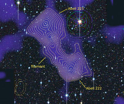
Fig. 6.59
The pair of clusters Abell 222 and 223, as
observed with the Subaru telescope, with the superimposed matter
distribution (blue shades
and yellow contours). The
filament between the pair of clusters is clearly indicated. Credit:
Jörg Dietrich, University of Michigan/University Observatory
Munich
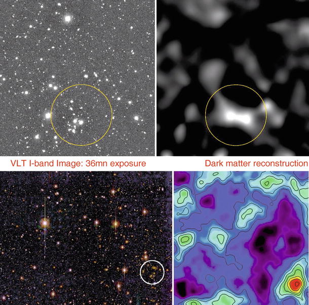
Fig. 6.60
Top
left: a VLT/FORS1 image, taken as part of a survey of ‘empty
fields’. Top right: the
mass reconstruction, as was obtained from the optical data by
employing the weak lensing effect. Clearly visible is a peak in the
mass distribution; the optical image shows a concentration of
galaxies in this region. Hence, in this field a cluster of galaxies
was detected for the first time by its lens properties.
Bottom: as above, here a
galaxy cluster was also detected through its lensing effect.
On the left, an optical
wide-field image is shown, obtained by the Big Throughput Camera,
and the mass reconstruction is displayed on the right. The location of the peak
in the latter coincides with a concentration of galaxies.
Spectroscopic measurements yield that these form a cluster of
galaxies at z = 0. 276.
Credit: Top: R. Maoli
et al., ESO. Bottom:
D. Wittman/Lucent Technologies’ Bell Labs, et al., NOAO, AURA,
NSF
Mass calibration
of clusters. We saw that the mass determination of clusters
from their X-ray emission is far from trivial, owing to the
complexity of the baryonic physics affecting the intracluster gas,
at least in the inner region of clusters. Any systematic
uncertainty in the mass estimate affects the scaling relations,
which are an essential tool for cluster cosmology (see
Sect. 8.2). Gravitational lensing offers
an alternative possibility for determining cluster masses which is
independent of equilibrium and symmetry assumptions. The accuracy
of weak lensing masses for individual clusters, out to large radii
(e.g., within r
500), is not impressive, and is affected by the noise
caused by intrinsic galaxy ellipticity, light deflection by other
masses along the line-of-sight to the source population, and the
mass-sheet degeneracy (see Problem 3.5). However, the mean
mass of a statistical sample of clusters can be obtained by using
the superposition of the individual lensing signals. The mass
estimate from such a ‘stacked’ cluster profile is viewed as being
least affected by systematic effects, and therefore frequently
employed in constructing scaling relations. In Sect. 7.7 we will present results of such
studies.
The search for
clusters of galaxies with weak gravitational lensing. The
weak lensing effect can not only be used to map the matter
distribution of known clusters, but it can also be employed to
search for clusters. Mass concentrations generate a tangentially
oriented shear field in their vicinity, which can specifically be
searched for. The advantage of this method is that it detects
cluster-mass matter concentrations based solely on their mass
properties, in contrast to all other methods which rely on the
emission of electromagnetic radiation, whether in the form of
optical light from cluster galaxies or as X-ray emission from a hot
intracluster medium. In particular, if clusters with atypically low
gas or galaxy content exist, they could be detected in this
way.
Quite a number of galaxy clusters have been
detected with this method—see Fig. 6.60. Further candidates
exist, where the shear signal indicates a significant mass
concentration but it cannot be identified with any concentration of
galaxies on optical images. The clarification of the nature of
these lens signals is of great importance: if in fact matter
concentrations do exist which correspond to the mass of a cluster
but which do not contain luminous galaxies, then our understanding
of galaxy evolution needs to be revised. However, we cannot exclude
the possibility that these statistically significant signals are
statistical outliers, or result from projection effects—remember,
lensing probes the line-of-sight integrated matter density.
Together with the search for galaxy clusters by means of the
SZ-effect (Sect. 6.4.4), the weak lensing effect provides an
interesting alternative for the detection of mass concentrations
compared to the more traditional methods.
6.7 The galaxy population in clusters
6.7.1 Luminosity function of cluster galaxies
The luminosity function of galaxies in a cluster
is defined in a similar way as in Sect. 3.10 for the total galaxy
population. In many clusters, the Schechter luminosity
function (3.52) represents a good fit to the
data if the brightest galaxy is disregarded in each cluster (see
Fig. 3.51 for the Virgo cluster of
galaxies). The slope α at
the faint end is not easy to determine, since projection effects
become increasingly important for fainter galaxies. The value of
α seems to vary between
clusters, but it is not entirely clear whether this result may also
be affected by projection effects of differing strength in
different clusters. Thus, no final conclusion has been reached as
to whether the luminosity function has a steep increase at
L ≪ L ∗ or not, i.e., whether
many more faint galaxies exist than
luminous ∼ L∗-galaxies (compare the galaxy content in
the Local Group, Sect. 6.1.1, where even in our close neighborhood it
is difficult to obtain a complete census of the galaxy population).
L ∗ is very
similar for many clusters, which is the reason why the distance
estimate by apparent brightness of cluster members, as done by
Abell for his cluster catalog, is quite reliable, though a number
of clusters exists with a clearly deviating value of L ∗.
However, when averaging over many clusters, the
picture becomes much clearer. The luminosity function of galaxies
changes as one moves from field galaxies, through groups, to
clusters. This change is already noticeable for poor groups with
just a few galaxies, such as the Local Group. The faint-end slope
of the luminosity function is flatter in group and cluster
environments than for field galaxies, and flattens with increasing
cluster mass or richness. Most galaxies with L ≲ L ∗ live either in isolation
or in relatively poor groups, whereas the most luminous galaxies
are predominantly found in the central regions of rich groups and
clusters. Whereas the fraction of elliptical galaxies is much
smaller in low-density regions than in the inner part of clusters,
they nevertheless dominate the galaxy mix at the highest
luminosities.
Brightest Cluster
Galaxies. Of special interest in clusters is the Brightest
Cluster Galaxy (BCG), which in most cases is located near the
center of the cluster. In many cases, the BCG is a cD galaxy; these differ from large
ellipticals in several respects. They have a very extended stellar
envelope, whose size may exceed R ∼ 100 kpc and whose surface
brightness profile is much broader than that of a de
Vaucouleurs-profile (see Fig. 3.11). cD galaxies are found only in
the centers of clusters or groups, thus only in regions of strongly
enhanced galaxy density. However, the extended stellar envelope
merges into the intracluster light, and there is some ambiguity to
distinguish between cD envelope and ICL, as discussed in
Sect. 6.3.4.
Many cD galaxies have multiple cores, which is a rather rare
phenomenon among the other cluster members.
BCGs are very luminous and massive; their typical
stellar mass is  ,
with a spread of about a factor of 1.5. One finds that the more
massive clusters contain the more luminous BCGs. At first sight,
this is not too surprising, since the more galaxies a cluster
contains, the larger is the probability to find one of them with
very high stellar mass (or luminosity). However, there are several
indications that this cannot be the sole reason. First, in most
clusters, the second brightest cluster galaxy is about 1 mag or
more fainter than the BCG, which cannot be explained purely by
statistical arguments. Second, the BCGs appear to be not simply the
extension of early-type galaxies towards the highest luminosity;
for example, BCGs do not fall right on the fundamental plane for
ellipticals. Their size-luminosity relation is different from that
of ellipticals, in the sense that they are larger than ellipticals
with the sameluminosity.
,
with a spread of about a factor of 1.5. One finds that the more
massive clusters contain the more luminous BCGs. At first sight,
this is not too surprising, since the more galaxies a cluster
contains, the larger is the probability to find one of them with
very high stellar mass (or luminosity). However, there are several
indications that this cannot be the sole reason. First, in most
clusters, the second brightest cluster galaxy is about 1 mag or
more fainter than the BCG, which cannot be explained purely by
statistical arguments. Second, the BCGs appear to be not simply the
extension of early-type galaxies towards the highest luminosity;
for example, BCGs do not fall right on the fundamental plane for
ellipticals. Their size-luminosity relation is different from that
of ellipticals, in the sense that they are larger than ellipticals
with the sameluminosity.6.7.2 The morphology-density relation
As mentioned several times before, the mixture of
galaxy types in clusters seems to differ from that of isolated
(field) galaxies. Whereas about 70 % of luminous field galaxies are
spirals, clusters are dominated by early-type galaxies, in
particular in their inner regions. Furthermore, the fraction of
spirals in a cluster depends on the distance from the center and
increases for larger r.
Obviously, the local density has an effect on the morphological mix
of galaxies. As in clusters, the fraction of group members which
are spirals is lower than the fraction of spirals among field
(i.e., isolated) galaxies, and the relative abundance of spiral
galaxies decreases with increasing σ v of the group.
More generally, one may ask whether the mixture
of the galaxy population depends on the local galaxy density. While
earlier studies of this effect were frequently confined to galaxies
within and around clusters, extensive redshift surveys like the
2dFGRS and the SDSS (see Sect. 8.1.2) allow us to systematically
investigate this question with very large and carefully selected
samples of galaxies. The morphological classification of such large
samples is performed by automated software tools, which basically
measure the light concentration in the galaxies, or, alternatively,
the best-fitting Sérsic-index n [see (3.39)]. A comparison of galaxies
classified this way with visual classifications shows very good
agreement.
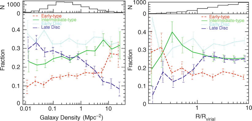
Fig. 6.61
The number fraction of galaxies of
different morphologies is plotted as a function of the local galaxy
density (left panel), and
for galaxies in clusters as a function of the distance from the
cluster center, scaled by the corresponding virial radius
(right panel). Galaxies are
divided into four different classes. ‘Early-types’ contain mainly
ellipticals, ‘intermediates’ are mainly S0-galaxies, ‘early and
late discs’ are predominantly Sa- and Sc-spirals, respectively. In
both representations, a clear dependence of the galaxy mix on the
density or on the distance from the cluster center, respectively,
is visible. In the histograms at the top of each panel, the number
of galaxies in the various bins is plotted. Source: T. Goto
et al. 2003, The
morphology-density relation in the Sloan Digital Sky Survey,
MNRAS 346, 601, p. 607, 608, Figs. 12, 15. Reproduced by
permission of Oxford University Press on behalf of the Royal
Astronomical Society
Results from the
Sloan Digital Sky Survey. As an example of such an
investigation, results from the Sloan Digital Sky Survey are shown
in Fig. 6.61.
Galaxies were morphologically classified, based on SDSS photometry,
and separated into four classes, corresponding to elliptical
galaxies, S0-galaxies, and early (Sa) and late (Sc) types of
spiral. In this analysis, only galaxies were included for which the
redshift was spectroscopically measured. Therefore, the spatial
galaxy density can be estimated. However, one needs to take into
account the fact that the measured redshift is a superposition of
the cosmic expansion and the peculiar velocity of a galaxy. The
peculiar velocity may have rather large values ( ∼ 1000 km∕s), in
particular in clusters of galaxies. For this reason, for each
galaxy in the sample the surface number density of galaxies which
have a redshift within ± 1000 km∕s of the target galaxy was
determined. The left panel in Fig. 6.61 shows the fraction
of the different galaxy classes as a function of this local galaxy
density. A very clear dependence, in particular of the fraction of
late-type spirals, on the local density can be seen: in regions of
higher galaxy density Sc-spirals contribute less than 10 % of the
galaxies, whereas their fraction is about 30 % in low-density
regions. Combined, the fraction of spirals decreases from ∼ 65 % in
the field to about 35 % in regions of high galaxy density. In
contrast, the fraction of ellipticals and S0-galaxies increases
towards higher densities, with the increase being strongest for
ellipticals.
In the right-hand panel of Fig. 6.61, the mixture of
galaxy morphologies is plotted as a function of the distance to the
center of the nearest cluster, where the distance is scaled by the
virial radius of the corresponding cluster. As expected, a very
strong dependence of the fraction of ellipticals and spirals on
this distance is seen. Sc-spirals contribute a mere 5 % of galaxies
in the vicinity of cluster centers, whereas the fraction of
ellipticals and S0-galaxies strongly increases inwards.
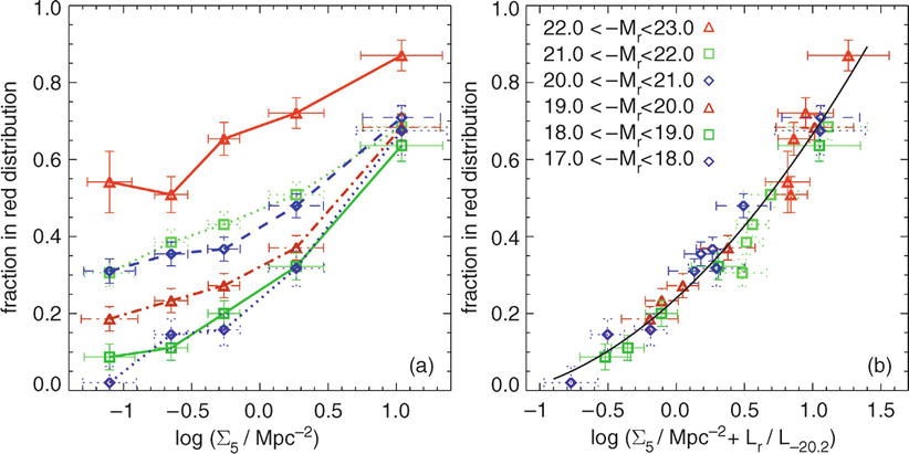
Fig. 6.62
On the
left, the fraction of galaxies in the red population (see
Sect. 3.1.3) is shown as a function of
Σ 5, an
estimator of the local galaxy number density based on the projected
distance of the fifth-nearest spectroscopically confirmed neighbor
galaxy within ± 1000 km∕s. Different symbols correspond to
different luminosity bins, as indicated. On the right, the same red fraction is
plotted against a combination of the local galaxy density
Σ 5 and the
luminosity of the galaxy. Source: I.K. Baldry et al. 2004,
Color bimodality: Implications for
galaxy evolution, astro-ph/0410603, Fig. 6. Reproduced by
permission of the author
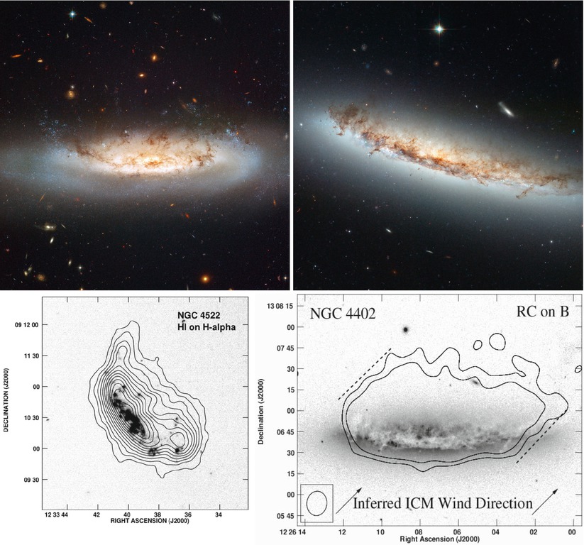
Fig. 6.63
Two edge-on spiral galaxies in the Virgo
cluster, NGC 4522 (left)
and NGC 4402 (right). The
top panels show multi-color
composite images of these two galaxies, taken with the HST. The
high velocity of the galaxies moving through the intracluster gas
removes part of the interstellar medium through ram pressure
stripping; in addition, the interaction of the intracluster gas
with the ISM of the galaxies triggers star formation, as can be
seen by the blue knots of emission downstream (i.e., above the
disk). The bottom panels
show the neutral hydrogen gas (left, for NGC 4522) and the 20 cm radio
emission (right, for
NGC 4022) of these two galaxies (note that the orientation of these
images are different from those of the HST images). The gas is
distributed asymmetrically with respect to the galactic disk,
emphasizing the stripping of gas from the galaxies. In the
bottom right, the
arrows indicate the
direction of the ICM velocity as seen in the rest-frame of the
galaxy (i.e., the galaxy moves in the opposite direction to these
arrows). Credit:
Top panels: NASA & ESA.
Bottom left: B. Vollmer
et al. 2008, Ram-pressure
stripped molecular gas in the Virgo spiral galaxy NGC 4522,
A&A 491, 455, p. 461, Fig. 13. ©ESO. Reproduced with
permission. Bottom right: H.H. Crowl 2005, Dense Cloud Ablation and Ram Pressure
Stripping of the Virgo Spiral NGC 4402, AJ 130, 65,
p. 68, Fig. 3. ©AAS. Reproduced with permission
Fig. 6.64
The left
panel shows an XMM-Newton image of the cluster Abell 3627.
On the right, the region
highlighted in the left
panel is zoomed in, showing the X-ray emission as observed
with Chandra (in blue), a
narrow-band optical image centered on the Hα line in red, both of which are superposed on
the broad-band optical image of the cluster (in white; obtained with the SOAR telescope
in Chile). The X-ray image clearly shows two tails, with some
80 kpc length, originating from the galaxy ESO 137-001 located on
the left in this image. These tails are generated by ram-pressure
stripping caused by the hot intracluster medium (seen through its
X-ray emission in the left
panel), as the galaxy moves towards the central region of
the cluster. The stripped gas is heated to temperatures of ∼ 1 keV,
about a factor of 10 smaller than the temperature of the hot
intracluster medium. The Hα
emission is mainly caused by H ii regions and thus indicates
regions of star formation. Hence, new stars are formed in the gas
that is removed from the galaxy. These stars will contribute to the
intracluster light. Furthermore, 19 X-ray point sources were found
around the X-ray tails, some of them being candidates for
ultra-luminous X-ray sources (ULX). Together, this observation
shows a clear connection between the evolution of galaxies in
clusters and the intracluster medium. Credit: X-ray:
NASA/CXC/UVa/M. Sun, et al.; H-alpha/Optical: SOAR
(UVa/NOAO/UNC/CNPq-Brazil). Corresponding journal article:
M. Sun et al. 2010, Spectacular X-ray Tails, Intracluster Star
Formation, and ULXs in A3627, ApJ 708, 946, p. 949,
Fig. 2. ©AAS. Reproduced with permission
The two diagrams in Fig. 6.61 are of course not
mutually independent: a region of high galaxy density is very
likely to be located in the vicinity of a cluster center, and the
opposite is valid accordingly. Therefore, it is not immediately
clear whether the mix of galaxy morphologies depends primarily on
the respective density of the environment of the galaxies, or
whether it is caused by morphological transformations in the inner
regions of galaxy clusters.
The morphology-density relation is also seen in
galaxy groups. The fraction of late-type galaxies decreases, and
the fraction of early-type galaxies increases with decreasing
distance from the group center, as is also the case in clusters.
When considering the morphological mix of visually classified
early- and late-type galaxies, averaged over the whole group or
cluster, i.e., up to the virial radius, then it seems to be
constant for group/cluster halo masses in excess of  .
.
.Alternative
consideration: the color-density relation. We pointed out in
Sect. 3.1.3 that galaxies at fixed
luminosity seem to have a bimodal color distribution (see
Fig. 3.7). Using the same data set as
that used for Fig. 3.7, the fraction of galaxies that
are contained in the red population can be studied as a function of
the local galaxy density. The result of this study is shown in the
left-hand panel of Fig. 6.62, where the fraction of galaxies belonging
to the red population is plotted against the local density of
galaxies, measured in terms of the fifth-nearest neighboring galaxy
within a redshift of ± 1000 km∕s. The fraction of red galaxies
increases towards higher local number density, and the relative
increase is stronger for the less luminous galaxies. If we identify
the red galaxies with the early-type galaxies in Fig. 6.61, these two results
are in qualitative agreement. Surprisingly, the fraction of
galaxies in the red sample seems to be a function of a combination
of the local galaxy density and the luminosity of the galaxy, as is
shown in the right-hand panel of Fig. 6.62.
Interpretation. A closer examination of
Fig. 6.61 may
provide a clue as to what physical processes are responsible for
the dependence of the morphological mix on the local number
density. We consider first the right-hand panel of
Fig. 6.61.
Three different regimes in radius can be identified: for
 , the fraction of the
different galaxy types remains basically constant. In the
intermediate regime,
, the fraction of the
different galaxy types remains basically constant. In the
intermediate regime,  , the
fraction of S0-galaxies strongly increases inwards, whereas the
fraction of late-type spirals decreases accordingly. This result is
compatible with the interpretation that in the outer regions of
galaxy clusters spirals lose gas, for instance by their motion
through the intergalactic medium (see Fig. 6.63), and these galaxies
then transform into passive S0-galaxies. Below
, the
fraction of S0-galaxies strongly increases inwards, whereas the
fraction of late-type spirals decreases accordingly. This result is
compatible with the interpretation that in the outer regions of
galaxy clusters spirals lose gas, for instance by their motion
through the intergalactic medium (see Fig. 6.63), and these galaxies
then transform into passive S0-galaxies. Below  , the fraction of
S0-galaxies decreases strongly, and the fraction of ellipticals
increases substantially.
, the fraction of
S0-galaxies decreases strongly, and the fraction of ellipticals
increases substantially.
, the fraction of the
different galaxy types remains basically constant. In the
intermediate regime, , the
fraction of S0-galaxies strongly increases inwards, whereas the
fraction of late-type spirals decreases accordingly. This result is
compatible with the interpretation that in the outer regions of
galaxy clusters spirals lose gas, for instance by their motion
through the intergalactic medium (see Fig. 6.63), and these galaxies
then transform into passive S0-galaxies. Below , the fraction of
S0-galaxies decreases strongly, and the fraction of ellipticals
increases substantially.In fact, the ratio of the number densities of
S0-galaxies and ellipticals, for  , strongly decreases
as R decreases. This may
hint at a morphological transformation in which S0 galaxies are
turned into ellipticals, probably by collisions or mergers. Such
gas-free mergers, also called ‘dry mergers’ , may be the preferred
explanation for the generation of elliptical galaxies. One of the
essential properties of dry mergers is that such a merging process
would not be accompanied by a burst of star formation, unlike the
case of gas-rich collisions of galaxies. The existence of a
population of newly-born stars in ellipticals would be difficult to
reconcile with the generally old stellar population actually
observed in these galaxies. We will discuss these issues more
thoroughly in Chap. 10.
, strongly decreases
as R decreases. This may
hint at a morphological transformation in which S0 galaxies are
turned into ellipticals, probably by collisions or mergers. Such
gas-free mergers, also called ‘dry mergers’ , may be the preferred
explanation for the generation of elliptical galaxies. One of the
essential properties of dry mergers is that such a merging process
would not be accompanied by a burst of star formation, unlike the
case of gas-rich collisions of galaxies. The existence of a
population of newly-born stars in ellipticals would be difficult to
reconcile with the generally old stellar population actually
observed in these galaxies. We will discuss these issues more
thoroughly in Chap. 10.Considering now the dependence on local galaxy
density (the left-hand panel of Fig. 6.61), a similar behavior
of the morphological mix of galaxies is observed: there seem to
exist two characteristic values for the galaxy density where the
relative fractions of galaxy morphologies change noticeably.
Interestingly, the relation between morphology and density seems to
evolve only marginally between z = 0. 5 and the local Universe.
One clue as to the origin of the morphological
transformation of galaxies in clusters, as a function of distance
from the cluster center, comes from the observation that the
velocity dispersion of very bright cluster galaxies seems to be
significantly smaller than that of less luminous ones. Assuming
that the mass-to-light ratio does not vary substantially among
cluster members, this then indicates that the most massive galaxies
have smaller velocity dispersions. One way to achieve this trend in
the course of cluster evolution is by dynamical interactions
between cluster galaxies. Such interactions tend to ‘thermalize’
the velocity distribution of galaxies, so that the mean kinetic
energy of galaxies tends to become similar. This then causes more
massive galaxies to become slower on average. If this
interpretation holds, then the morphology-density relation may be
attributed to these dynamical interactions, rather than to the
(so-called ram-pressure) stripping of the interstellar medium as
the galaxies move through the intracluster medium.
However, ram-pressure stripping of the
interstellar medium has been clearly observed in clusters. In
Fig. 6.63,
two edge-on spiral galaxies in the Virgo cluster are shown, both in
the optical and in the radio. The impact of the intracluster
medium, which acts like a ‘wind’ in the rest-frame of the galaxies,
can be clearly seen. This effect mostly acts on the atomic gas of
spirals, whereas the molecular gas seems to be less affected; we
recall that the molecular gas is more densely concentrated towards
the galactic disk, and thus more strongly bound. In fact, it has
been known for a long time that there are spiral galaxies in groups
and clusters which are deficient in neutral hydrogen, relative to
field galaxies of the same stellar luminosity. If ram-pressure
stripping, or other effects in the dense cluster environment,
removes the interstellar medium from spirals, then the result could
be a disk galaxy without ongoing star formation—something that may
resemble an S0-galaxy. If that were the case, than S0s would be
passively fading former spirals. Whereas the original spirals
satisfied the Tully–Fisher relation, the S0s would then be expected
to be considerably fainter than spirals, at fixed rotational
velocity; this indeed is the case.
Fig. 6.65
X-ray luminosity function of galaxy
clusters, as was obtained from a region around the north ecliptic
pole (NEP), the region with the longest exposure time in the ROSAT
All-Sky Survey (see Fig. 6.40). Plotted is dN∕dL X, the (comoving) number
density per luminosity interval, for clusters with
0. 02 ≤ z ≤ 0. 3
(left panel) and
0. 3 ≤ z ≤ 0. 85
(right panel),
respectively. The luminosity was derived from the flux in the
photon energy range from 0.5 to 2 keV. The three different curves specify the
local luminosity function of clusters as found in other cluster
surveys at lower redshifts. We see that evolutionary effects in the
luminosity function are relatively small and become visible only at
high L X.
Source: I.M. Gioia et al. 2001, Cluster Evolution in the ROSAT North Ecliptic
Pole Survey, ApJ 553, L105, p. L106, Fig. 1. ©AAS.
Reproduced with permission
Ram-pressure stripping not only removes gas from
cluster galaxies, but can heat the gas and also trigger local star
formation, though the compression of gaseous regions by the
pressure. A spectacular example for this is shown in
Fig. 6.64.
The newly formed stars are no longer gravitationally bound to the
galaxy, and will thus contribute to the ICL in the cluster.
E + A
galaxies. Galaxy clusters
contain a class of galaxies which is defined in terms of spectral
properties. These galaxies, which are rare in number, show strong
Balmer line absorption in their spectra, characteristic of A stars,
but no [Oii] or
Hα emission lines. The
latter indicates that these galaxies are not undergoing strong star
formation at present (since there are no Hii regions around O- and B-stars),
whereas the former shows that there was an episode of star
formation within the past ∼ 1 Gyr, about as long ago as the
main-sequence lifetime of A stars. These galaxies have been termed
E + A galaxies since their spectra appears like a superposition of
that of A-stars and that of otherwise normal elliptical galaxies.
They are interpreted as being post-starburst galaxies. Since they
were first seen in clusters, the interpretation of the origin of E
+ A galaxies was originally centered on the cluster environment—for
example star-forming galaxies falling into a cluster and having
their interstellar medium removed by tidal forces caused by the
cluster potential well and/or stripping as the galaxies move
through the intracluster medium. However, E + A galaxies were later
also found in different environments, making the above
interpretation largely obsolete. By investigating the spatial
correlation of these galaxies with other galaxies shows that the
phenomenon is not associated with the large-scale environment. An
overdensity of neighboring galaxies can be seen only out to scales
of ∼ 100 kpc. If the sudden turn-off of the star-formation activity
is indeed caused by an external perturbation, it is therefore
likely that it is caused by the dynamical interaction of close
neighboring galaxies or by mergers. Indeed, about 30 % of E + A
galaxies are found to have morphological signatures of
perturbations, such as tidal tails, supporting the interaction
hypothesis.
In fact, the spiral galaxies in clusters seem to
differ statistically from those of field spirals, in that the
fraction of disk galaxies with absorption-line spectra, and thus no
ongoing star formation, seems to be larger in clusters than in the
field by a factor ∼ 4, indicating that the cluster environment has
a marked impact on the star-formation ability of these
galaxies.
6.8 Evolutionary effects
Today, we are able to discover and analyze
clusters of galaxies at redshifts z ∼ 1 and higher; thus the question
arises whether these clusters have the same properties as local
clusters. At z ∼ 1 the age
of the Universe is only about half of that of the current Universe.
One might therefore expect an evolution of cluster
properties.
Luminosity
function. First, we shall consider the comoving number
density of clusters as a function of redshift or, more precisely,
the evolution of the luminosity function of clusters with
z. As Fig. 6.65 demonstrates, such
evolutionary effects are not very pronounced for moderate
redshifts, and only at the highest luminosities or the most massive
clusters, respectively, does an evolution become visible. The
situation is somewhat different when one considers the evolution of
the cluster abundance as a function of temperature: at redshift
z ∼ 0. 5, the number of
clusters above a given temperature is lower than at the current
epoch by a factor ∼ 3. Hence, there obviously is an evolution of
the cluster population, in the sense that at high redshift,
clusters of very high luminosity, high temperature, or very high
mass are less abundant than they are today. The interpretation and
the relevance of this fact will be discussed later (see
Sect. 8.2.1). We also note that a weak
redshift evolution of the X-ray luminosity function of clusters is
compatible with a strong evolution of the cluster mass function,
since according to (6.62), the relation between luminosity and mass
evolves significantlywith z
Butcher–Oemler
effect. We saw in Chap. 3 that early-type galaxies are
predominantly found in clusters and groups, whereas spirals are
mostly field galaxies. For example, a massive cluster like Coma
contains only 10 % spirals, the other luminous galaxies are
ellipticals or S0 galaxies (see also Sect. 6.7.2). Besides these
morphological differences, the colors of galaxies are very useful
for a characterization: early-type galaxies (ellipticals and S0
galaxies) have little ongoing star formation and therefore consist
mainly of old, thus low-mass and cool stars. Hence they are red,
whereas spirals feature active star formation and are therefore
distinctly bluer. The fraction of blue galaxies in nearby clusters
is very low.
Fig. 6.66
Butcher–Oemler effect: in the upper panel, the fraction of blue
galaxies f b in
a sample of 195 galaxy clusters is plotted as a function of cluster
redshift, where open
(filled) circles indicate photometric
(spectroscopic) redshift data for the clusters. The lower panel shows a selection of
clusters with spectroscopically determined redshifts and
well-defined red cluster sequence. For the determination of
f b, foreground
and background galaxies need to be statistically subtracted using
control fields, which can also result in negative values for
f b. A clear
increase in f b
with redshift is visible, and a line of regression yields
 . Source: V.E.
Margoniner et al. 2001, The
Butcher-Oemler Effect in 295 Clusters: Strong Redshift Evolution
and Cluster Richness Dependence, ApJ 548, L143,
p. L144, Fig. 1. ©AAS. Reproduced with permission
. Source: V.E.
Margoniner et al. 2001, The
Butcher-Oemler Effect in 295 Clusters: Strong Redshift Evolution
and Cluster Richness Dependence, ApJ 548, L143,
p. L144, Fig. 1. ©AAS. Reproduced with permission
. Source: V.E.
Margoniner et al. 2001, The
Butcher-Oemler Effect in 295 Clusters: Strong Redshift Evolution
and Cluster Richness Dependence, ApJ 548, L143,
p. L144, Fig. 1. ©AAS. Reproduced with permissionButcher and Oemler found that this changes if one
examines clusters of galaxies at higher redshifts: these contain a
larger fraction of blue galaxies, thus of spirals (see
Fig. 6.66).
This means that the mixture of galaxies changes over time. In
clusters, spirals must become scarcer with increasing cosmic time,
e.g., by transforming into early-type galaxies. With 8-m class
telescopes, such studies can be extended to much higher redshifts.
It was found that the fraction of blue galaxies increases further,
until at z ≳ 1. 3 the blue
fraction in clusters is essentially the same as in the field.
A possible and plausible explanation is that
spirals lose their interstellar gas through ram-pressure stripping
(Fig. 6.63),
which is then mixed with the ICM. This is plausible because the ICM
also has a high metallicity. These metals can only originate in a
stellar population, thus in the enriched material in the ISM of
galaxies.
Indeed, from the colors of cluster galaxies it is
possible to derive very strict upper limits on their star formation
in recent times. The color of cluster galaxies at high redshifts
even provides interesting constraints on cosmological
parameters—only those models are acceptable which have an age of
the Universe, at the respective redshift, larger than the estimated
age of the stellar population. One interesting example of this is
presented in Fig. 6.67.
Therefore, we conclude from these observations
that the stars in cluster galaxies formed at very early times in
the Universe . But this does not necessarily mean that the galaxies
themselves are also this old, because galaxies can be transformed
into each other by merger processes (see Fig. 6.68). This changes the
morphology of galaxies, but may leave the stellar populations
largely unchanged.
At higher redshift (say, z ≳ 0. 5), the fraction of clusters
which show a cool core and which are therefore believed to be
relaxed is smaller than in the current Universe. This observational
finding is not unexpected, since the age of the Universe was
smaller back then, and thus there was considerably less time for
clusters to settle into an equilibrium state. Furthermore, the
metallicity of the intracluster gas decreases towards higher
redshifts, indicating that the enrichment of the gas is an ongoing
process.
Fig. 6.67
The radio galaxy LBDS 53W091 has a redshift
of z = 1. 552, and it
features a very red color (R − K ≈ 5. 8). Optical spectroscopy of the
galaxy provides us with the spectral light distribution of the UV
emission in the galaxy’s rest frame. The UV light of a stellar
population is almost completely due to stars on the upper main
sequence—see Fig. 3.34. In the upper left panel, the spectrum of
LBDS 53W091 is compared to those of different F stars; one can see
that F6 stars match the spectral distribution of the galaxy nearly
perfectly. In the bottom
panel, synthetic spectra from population synthesis
calculations are compared to the observed spectrum. A population
with an age of about 4 Gyr represents the best fit to the observed
spectrum; this is also comparable to the lifetime of F6 stars: the
most luminous (still existing) stars dominate the light
distribution of a stellar population in the UV. In combination,
this reveals that this galaxy at z = 1. 552 is at least 3 Gyr old.
Phrased differently, the age of the Universe at z = 1. 55 must be at least 3 Gyr. In
the upper right panel, the
age of the Universe at z = 1. 55 is displayed as a function of
H 0 and
Ω Λ (for  ).
Hence, this single galaxy provides significant constraints on
cosmological parameters. Source: H. Spinrad et al. 1997,
LBDS 53W091: an Old, Red Galaxy at
z = 1.552, ApJ 484, 581, p. 587, 595, 599, Figs. 8, 17,
18. ©AAS. Reproduced with permission
).
Hence, this single galaxy provides significant constraints on
cosmological parameters. Source: H. Spinrad et al. 1997,
LBDS 53W091: an Old, Red Galaxy at
z = 1.552, ApJ 484, 581, p. 587, 595, 599, Figs. 8, 17,
18. ©AAS. Reproduced with permission
).
Hence, this single galaxy provides significant constraints on
cosmological parameters. Source: H. Spinrad et al. 1997,
LBDS 53W091: an Old, Red Galaxy at
z = 1.552, ApJ 484, 581, p. 587, 595, 599, Figs. 8, 17,
18. ©AAS. Reproduced with permission
Fig. 6.68
The cluster of galaxies MS 1054−03,
observed with the HST, is the most distant cluster in the EMSS
X-ray survey (z = 0. 83).
The reddish galaxies in the image on the left form a nearly linear
structure. This cluster is far from being spherical, as we have
also seen from its weak lensing results (Fig. 6.55)—it is not relaxed.
The smaller images on the right show blow-ups of selected cluster
fields where mergers of galaxies become visible: in this cluster,
the merging of galaxies is directly observable. At least six of the
nine merging pairs found in this cluster have been shown to be
gravitationally bound systems. Credit: P. van Dokkum, M. Franx/U.
Groningen & U. Leiden, ESA, NASA
Clusters of
galaxies at very high redshift. The search for clusters at
high redshift is of great cosmological interest. As will be
demonstrated in Sect. 7.5.2, the expected number density
of clusters as a function of z strongly depends on the cosmological
model. Hence, this search offers an opportunity to constrain
cosmological parameters by the statistics of galaxy clusters.
The search for clusters in the optical (thus, by
galaxy overdensities) becomes increasingly difficult at high
z because of projection
effects. Nevertheless, several groups have managed to detect
clusters at z ∼ 0. 8 with
this technique. In particular, the overdensity of galaxies in
three-dimensional space can be analyzed if, besides the angular
coordinates on the sphere, the galaxy colors are also taken into
account. Because of the red cluster sequence , the overdensity is
much more prominent in this space than in the skyprojection
alone.
Fig. 6.69
The cluster of galaxies XMMU J2235.2−2557
was discovered in the field-of-view of an XMM-Newton image for
which a different source was the original target. The image
on the left shows the X-ray
contours, superposed on an R-band image, while the image
on the right shows the
central section, here superposed on a K-band image. Galaxies in the
field follow a red cluster sequence if the color is measured in
R − z. The symbols denote galaxies at redshift
1. 37 < z < 1. 40.
The strong X-ray source to the upper right of the cluster center is
a Seyfert galaxy at lower redshift. Until 2005, this cluster was
the most distant X-ray selected cluster known, with a temperature
of ∼ 6 keV and a velocity dispersion of σ ∼ 750 km∕s. Source: C.R. Mullis
et al. 2005, Discovery of an
X-Ray-luminous Galaxy Cluster at z=1.4, ApJ 623, L85,
p. L86, Fig. 1. ©AAS. Reproduced with permission
Fig. 6.70
A Ks-band image of the field
containing the cluster XMMXCS J2215.9−1738, superposed by the
contours of the X-ray emission observed with XMM-Newton. The
cluster was discovered by XMM-Newton as an extended X-ray source,
close to the center of this 3 ′ × 3 ′ field; the other three nearby
X-ray sources are unrelated point sources. The spectra of six
member galaxies identified this as a cluster at z = 1. 45, one of the highest redshift
X-ray detected clusters known. The temperature of the cluster is
measured to be ∼ 7 keV, signalling a very massive object, a
conclusion also obtained from the high X-ray luminosity. Source:
S.A. Stanford et al. 2006, The XMM Cluster Survey: A Massive Galaxy
Cluster at z = 1.45, ApJ 646, L13, p. L14, Fig. 1.
©AAS. Reproduced with permission
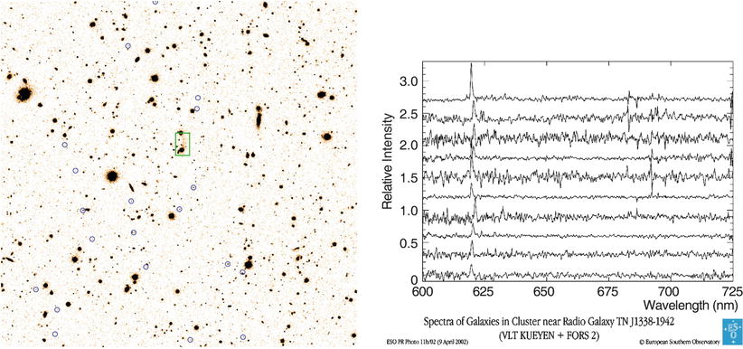
Fig. 6.71
The most distant known group of galaxies.
The region around the radio galaxy TN J1338−1942 (z = 4. 1) was scanned for galaxies at
the same redshift; 20 such galaxies were found with the VLT, marked
by circles in the left image. For ten of these
galaxies, the spectra are shown on
the right; in all of them, the Lyα emission line is clearly visible.
Hence, groups of galaxies were already formed in an early stage of
the Universe. Credits: B. Venemans, G. Miley et al., European
Southern Observatory
Projection effects play a considerably smaller
role in X-ray searches for clusters. With ROSAT, some clusters with
z ∼ 1. 2 were found (see
Fig. 6.39).
The current X-ray satellites Chandra and XMM-Newton are more
sensitive, and have detected several clusters with redshifts up to
2; two examples for clusters at z ∼ 1. 4 are shown in
Figs. 6.69
and 6.70. These examples demonstrate that combining
deep X-ray images with observations in the optical and the NIR is
an efficient method of compiling samples of distant clusters. More
recently, cluster detections using the Sunyaev–Zeldovich effect
have obtained an increasingly prominent role in finding
high-redshift clusters.
Through optical methods, it is also possible to
identify galaxy concentrations at very high redshift. One approach
is to assume that luminous AGNs at high redshift are found
preferentially in regions of high overdensity, which is also
expected from models of galaxy formation. With the redshift of the
AGN known, the redshift at which one should search for an
overdensity of galaxies near the AGN is defined. Those searches
have proven to be quite successful; for instance, they are
performed using narrow-band filter photometry, with the filter
centered on the redshifted Lyα line, tuned to the redshift of the
AGN. Candidates need to be verified spectroscopically afterwards.
One example of a strong galaxy concentration at z = 4. 1 is presented in
Fig. 6.71.
The identification of a strong spatial concentration of galaxies is
not sufficient to have identified a cluster of galaxies though,
because it is by no means clear whether one has found a
gravitationally bound system of galaxies (and the corresponding
dark matter). Rather, such galaxy concentrations are considered to
be the predecessors of galaxy clusters which will only evolve into
bound systems during later cosmological evolution; they are thus
often called ‘proto-clusters’.
6.9 Problems
6.1. The
virial radius. In Sect. 7.5.1 we will show, on the basis of
the spherical collapse model, that the mean density within a
virialized region is about 200 times the critical density of the
Universe at the time of collapse. We will derive here an
alternative and simple argument for that statement.
1.
Consider a circular orbit with radius
r 200 of a
particle in a dark matter halo of mass M 200. Calculate the orbital
time and show that it depends only on the mean density of the halo
inside the orbit,  .
Thus, this orbital time does not depend on the mass (or radius) of
the halo. Recall that the free-fall time t ff (see Problem 4.7)
has the same dependence on
.
Thus, this orbital time does not depend on the mass (or radius) of
the halo. Recall that the free-fall time t ff (see Problem 4.7)
has the same dependence on  —what is their ratio?
.
Thus, this orbital time does not depend on the mass (or radius) of
the halo. Recall that the free-fall time t ff (see Problem 4.7)
has the same dependence on —what is their ratio?2.
By setting the mean density to be 200ρ cr(z), show that the orbital time is, up
to a factor of order unity, the age of the Universe at the time of
the halo formation, i.e., the time of collapse!
Thus, for a halo characterized by a mean density
of 200 times the critical density ρ cr(z), a particle at the outer edge can
finish one orbit within the age of the Universe at redshift
z. Since the time scale for
relaxation cannot be smaller than the time a particle needs to
orbit through the region, the choice  is indeed
plausible.
is indeed
plausible.
is indeed
plausible.6.2. Cosmological surface brightness dimming.
Consider a source of bolometric luminosity L and radius R, and show that its bolometric surface
brightness decreases with redshift  . Calculate the redshift
dependence of the specific surface brightness I ν if the source has a power-law
spectrum, L
ν
∝ ν −α .
. Calculate the redshift
dependence of the specific surface brightness I ν if the source has a power-law
spectrum, L
ν
∝ ν −α .
. Calculate the redshift
dependence of the specific surface brightness I ν if the source has a power-law
spectrum, L
ν
∝ ν −α .Footnotes
1
Of course, the numbers quoted here are those of
currently known galaxies. Dwarf galaxies like Sagittarius would be
very difficult to detect at the distances of these groups.
2
The reason for choosing the third brightest
galaxy is that the luminosity of the brightest galaxy may vary
considerably among clusters. Even more important is the fact that
there is a finite probability for the brightest galaxy in a sky
region under consideration to not belong to the cluster, but to be
located at some smaller distance from us.
3
There are also other methods that have been used
to construct cluster catalogs, which run under name of ‘matched
filter’ techniques. They assume that galaxies are not only a
collection of galaxies, but that the galaxy overdensity has certain
properties. For example, the number density of cluster galaxies is
expected to have a particular radial density profile and their
distribution in luminosity should approximately follow a
Schechter-type luminosity function. Applying these criteria to
galaxy overdensities leads to cleaner cluster selection than a pure
overdensity criterion. As a drawback, these criteria are more
likely to select regular clusters than irregular ones, due to the
assumed density profile.
4
In principle, one might need more parameters for
describing the radial profile of clusters, and thus the parameters
mentioned are a bare minimum. However, as we shall see later, it
appears that the mass profiles of clusters are all very similar.
Cosmological simulations of structure evolution in the Universe
predict that the density profiles of clusters can indeed be
characterized by this minimum set.
6
The flatfield of an image (or, more precisely, of
the system consisting of telescope, filter, and detector) is
defined as the image of a uniformly illuminated field, so that in
the ideal case each pixel of the detector produces the same output
signal. This is not the case in reality, however, as the
sensitivity differs for individual pixels. For this reason, the
flatfield measures the sensitivity distribution of the pixels,
which is then accounted for in the image analysis.
7
We point out that the pair of (6.42)
and (6.43) is valid independently of the validity of
the assumptions from which (6.42) was obtained. If the observed X-ray
emission is very well described by (6.43), the gas density
profile (6.42) can be obtained from it, independently of
the validity of the assumptions made before.
8
One of the cluster catalogs that were extracted
from the RASS data is the HIFLUGCS catalog. It consists of the 63
X-ray-brightest clusters and is a strictly flux-limited survey,
with  ;
it excludes the Galactic plane, | b | ≤ 20∘, as well as other
regions around the Magellanic clouds and the Virgo cluster of
galaxies in order to avoid large column densities of Galactic gas
which lead to absorption, as well as Galactic and other nearby
X-ray sources. The extended HIFLUGCS survey contains, in addition,
several other clusters for which good measurements of the
brightness profile and the X-ray temperature are available.
;
it excludes the Galactic plane, | b | ≤ 20∘, as well as other
regions around the Magellanic clouds and the Virgo cluster of
galaxies in order to avoid large column densities of Galactic gas
which lead to absorption, as well as Galactic and other nearby
X-ray sources. The extended HIFLUGCS survey contains, in addition,
several other clusters for which good measurements of the
brightness profile and the X-ray temperature are available.9
It should be noted, though, that the
determination of L
X and M are
independent of each other, whereas in the mass determination the
temperature is an explicit parameter so that the measurements of
these two parameters are correlated.
10
Another lesson that can be learned from the
discovery of the arcs is one regarding the psychology of
researchers. After the first observations of arcs were published,
several astronomers took a second look at their own images of these
two clusters and clearly detected the arcs in them. The reason why
this phenomenon, which had been observed much earlier, was not
published before can be explained by the fact that researchers were
not completely sure about whether these sources were real. A
certain tendency prevails in not recognizing phenomena that occur
unexpectedly in data as readily as results which are expected.
However, there are also researchers who behave in exactly the
opposite manner and even interpret phenomena expected from theory
in some unusual way.
11
We will see in the next chapter that the density
of dark matter halos is predicted to increase right to the center,
i.e., no core is formed in this case.
12
Prominent examples for such cameras are Megacam
at CFHT, the first square degree camera with ∼ (18000)2
pixels, and OmegaCAM (with the same field-of-view) at the VLT
Survey Telescope on Paranal. The largest camera currently in
operation is that of Pan-STARRS1,
covering ∼ 6 deg2