The insight that our Milky Way is just one of many galaxies in the Universe is less than 100 years old, despite the fact that many had already been known for a long time. The catalog by Charles Messier (1730–1817), for instance, lists 103 diffuse objects. Among them M31, the Andromeda galaxy, is listed as the 31st entry in the Messier catalog. Later, this catalogue was extended to 110 objects. John Dreyer (1852–1926) published the New General Catalog (NGC) that contains nearly 8000 objects, most of them galaxies. Spiral structure in some of the nebulae was discovered in 1845 by William Parsons, and in 1912, Vesto Slipher found that the spiral nebulae are rotating, using spectroscopic analysis. But the nature of these extended sources, then called nebulae, was still unknown at that time; it was unclear whether they are part of our Milky Way or outside it.

The nature of the nebulae. The year 1920 saw a public debate (the Great Debate) between Harlow Shapley and Heber Curtis. Shapley believed that the nebulae are part of our Milky Way, whereas Curtis was convinced that the nebulae must be objects located outside the Galaxy. The arguments which the two opponents brought forward were partly based on assumptions which later turned out to be invalid, as well as on incorrect data. Much of the controversy can be traced back to the fact that at that time it was not known that dust in the Galactic disk leads to an extinction of distant objects. We will not go into the details of their arguments which were partially linked to the assumed size of the Milky Way since, only a few years later, the question of the nature of the nebulae was resolved.

In 1925, Edwin Hubble discovered Cepheids in Andromeda (M31). Using the period-luminosity relation for these pulsating stars (see Sect. 2.2.7) he derived a distance of 285 kpc. This value is a factor of ∼ 3 smaller than the distance of M31 known today, but it provided clear evidence that M31, and thus also other spiral nebulae, must be extragalactic. This then immediately implied that they consist of innumerable stars, like our Milky Way. Hubble’s results were considered conclusive by his contemporaries and marked the beginning of extragalactic astronomy. It is not coincidental that at this time George Hale began to arrange the funding for an ambitious project. In 1928 he obtained six million dollars for the construction of the 5 m telescope on Mt. Palomar which was completed in 1949.

Outline of this chapter. This chapter is about galaxies. We will confine the consideration here to ‘normal’ galaxies in the local Universe; galaxies at large distances, some of which are in a very early evolutionary state, will be discussed in Chap. 9, and active galaxies, like quasars for example, will be discussed later in Chap. 5 In Sect. 3.1, a classification scheme of galaxies that was introduced by Edwin Hubble will be described; most of the luminous galaxies in the local Universe find their place on this Hubble sequence of galaxies. The properties of the two main types of galaxies, elliptical and spiral galaxies, are then described in more detail in the following two sections. In Sect. 3.4, we will show that the parameters describing elliptical and spiral galaxies, such as mass, luminosity and size, have a quite regular distribution; the various galaxy properties are strongly mutually related, giving rise to so-called scaling relations.

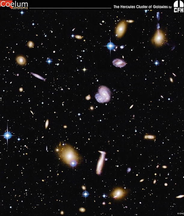
/epubstore/S/P-Schneider/Extragalactic-Astronomy-And-Cosmology/OEBPS/A129044_2_En_3_Fig1_HTML.jpg

Fig. 3.1

Galaxies occur in different shapes and sizes, and often they are grouped together in groups or clusters. This cluster, the Hercules cluster (also called Abell 2151), lies at a redshift of z = 0. 037 and contains numerous galaxies of different types and luminosities. The galaxies differ in their morphology, as well as in their colors—spiral galaxies are considerably bluer than elliptical galaxies. In the center of the image, an interacting pair of spiral galaxies (known as NGC 6050/IC 1179, or together as Arp 272) is visible. Credit: Canada-France-Hawaii Telescope/Coelum, Image by Jean-Charles Cuillandre (CFHT) & Giovanni Anselmi (Coelum)

We will then turn in Sect. 3.5 to investigating the stellar population of galaxies, in particular related to the question of whether the emitted spectral energy distribution of a galaxy can be understood as a sum of the emission of its stars, and how the spectrum of galaxies is related to the properties of the stellar population. The insights gained from that consideration allow us to understand and interpret the finding that the colors of galaxies fall mainly into two groups—they are either red or blue. As we shall see in Sect. 3.6, this offers an alternative classification scheme of galaxies which is independent of their morphology; this obviously comes in handy if one wants to classify galaxies at large distances for which morphological information is much more difficult to obtain, due to their small angular sizes on the sky. We will also see how this new classification fits together with the Hubble sequence.

After a short section on the chemical evolution of galaxies, we will describe in Sect. 3.8 evidence for the existence of supermassive black holes in the center of galaxies, with masses ranging up to 10⁹ M _⊙, and for a tight relation between the black hole mass and properties of the stellar component of the galaxies. We then turn to the question on how distances of galaxies can be measured directly, i.e., without employing the Hubble law (1.6). These distance determinations are required in order to calibrate the Hubble law, i.e., to determine the Hubble constant H ₀.

The distribution of galaxies in luminosity will be studied in Sect. 3.10; we will see that there exists a characteristic luminosity L ^∗ of galaxies, such that most of the stars in the current Universe are hosted by galaxies whose luminosity varies in a rather narrow interval around L ^∗. We will see towards the end of this book that the occurrence of this characteristic luminosity (or stellar mass) scale is one of the smoking guns for understanding the cosmic evolution of galaxies. In Sect. 3.11 we describe the gravitational lensing effects caused by massive galaxies, and study some of its applications.

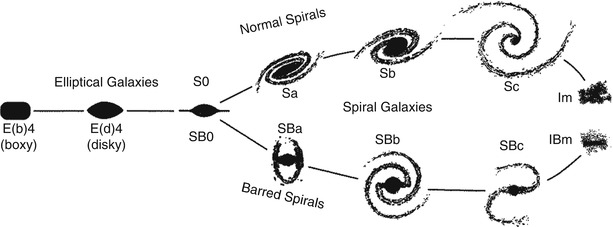
/epubstore/S/P-Schneider/Extragalactic-Astronomy-And-Cosmology/OEBPS/A129044_2_En_3_Fig2_HTML.jpg

Fig. 3.2

Hubble’s ‘tuning fork’ for galaxy classification. Adapted from: J. Kormendy & R. Bender 1996, A Proposed Revision of the Hubble Sequence for Elliptical Galaxies, ApJ 464, L119, Fig. 1. ©AAS. Reproduced with permission

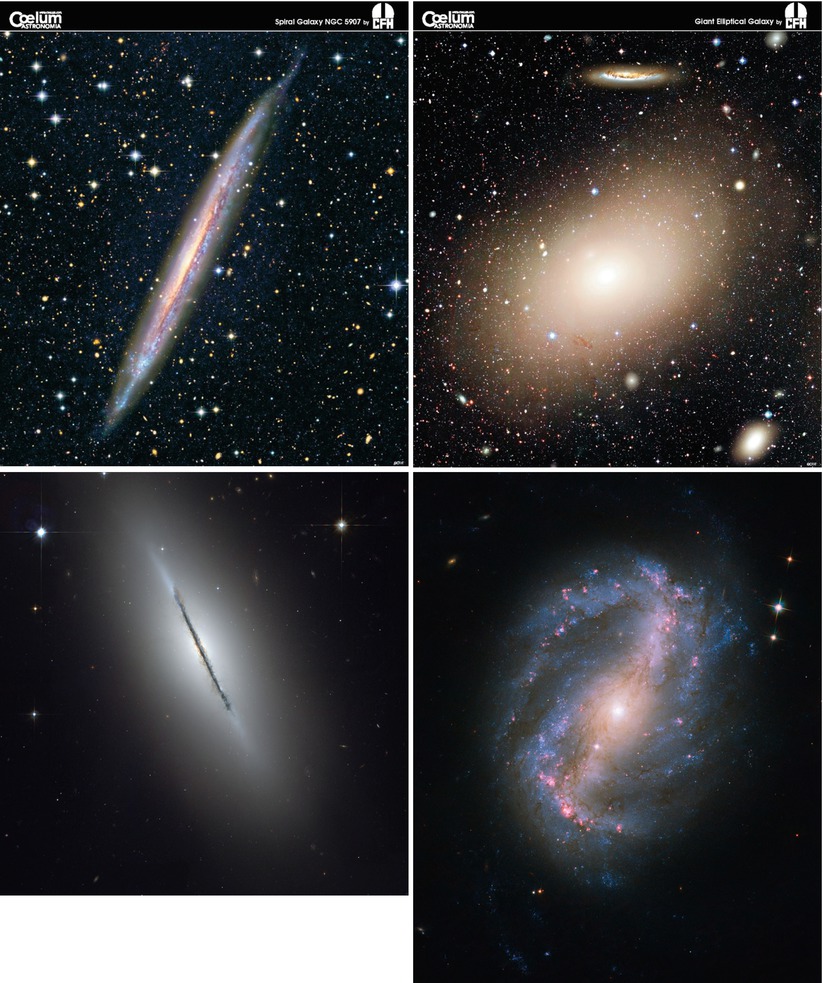
/epubstore/S/P-Schneider/Extragalactic-Astronomy-And-Cosmology/OEBPS/A129044_2_En_3_Fig3_HTML.jpg

Fig. 3.3

Four galaxies at different locations on the Hubble sequence. NGC 5907 (top left) is a large edge-on spiral galaxy whose dust layer inside the stellar disk is seen due to its reddening effect. In contrast, NGC 5866 is an edge-on S0 (lenticular) galaxy (bottom left) though a thin disk is visible like in the edge-on spiral galaxy, the morphology is clearly distinct. The top right image shows the giant elliptical galaxy M86 located in the Virgo cluster of galaxies, whereas the bottom right panel displays the barred spiral galaxy NGC 6217. Credits: Top right and left: Canada-France-Hawaii Telescope/Coelum, Image by Jean-Charles Cuillandre (CFHT) & Giovanni Anselmi (Coelum). Bottom left: NASA, ESA, and The Hubble Heritage Team (STScI/AURA), W. Keel (University of Alabama, Tuscaloosa). Bottom right: NASA, ESA, and the Hubble SM4 ERO Team

3.1 Classification

Galaxies are observed to have a variety of properties (see Fig. 3.1)—shapes, luminosities, colors, metallicities, etc. The classification of objects depends on the type of observation according to which this classification is made. This is also the case for galaxies. Historically, optical photometry was the method used to observe galaxies. Thus, the morphological classification defined by Hubble is still the best-known today. Besides morphological criteria, color indices, spectroscopic parameters (based on emission or absorption lines), the broad-band spectral distribution (galaxies with/without radio- and/or X-ray emission, or emission in the infrared), as well as other features may also be used.

We start with the Hubble sequence of galaxies, before briefly mention in Sect. 3.1.2 other types of galaxies which do not fit into the Hubble sequence, and outline an alternative classification scheme in Sect. 3.1.3.

3.1.1 Morphological classification: The Hubble sequence

Figure 3.2 shows the classification scheme defined by Hubble. According to this, three main types of galaxies exist (see also Fig. 3.3 for examples):

Elliptical galaxies (E’s) are galaxies that have nearly elliptical isophotes¹ without any clearly defined structure. They are subdivided according to their ellipticity $\epsilon \equiv 1 - b/a$ , where a and b denote the semi-major and the semi-minor axes, respectively. Ellipticals are found over a relatively broad range in ellipticity, $0 \leq \epsilon \lesssim 0.7$ . The notation En is commonly used to classify the ellipticals with respect to ε, with n = 10ε; i.e., an E4 galaxy has an axis ratio of , and E0’s have circular isophotes.
Spiral galaxies consist of a disk with spiral arm structure and a central bulge. They are divided into two subclasses: normal spirals (S’s) and barred spirals (SB’s). In each of these subclasses, a sequence is defined that is ordered according to the brightness ratio of bulge and disk, and that is denoted by a, ab, b, bc, c, cd, d. Objects along this sequence are often referred to as being either an early-type or a late-type; hence, an Sa galaxy is an early-type spiral, and an SBc galaxy is a late-type barred spiral. We stress explicitly that this nomenclature is not a statement of the evolutionary stage of the objects but is merely a nomenclature of purely historical origin.
Irregular galaxies (Irr’s) are galaxies with only weak (Irr I) or no (Irr II) regular structure. The classification of Irr’s is often refined. In particular, the sequence of spirals is extended to the classes Sdm, Sm, Im, and Ir (m stands for Magellanic; the Large Magellanic Cloud is of type SBm).
S0 galaxies are a transition between ellipticals and spirals which are also called lenticulars as they are lentil-shaped galaxies. They contain a bulge and a large enveloping region of relatively unstructured brightness which often appears like a disk without spiral arms. Ellipticals and S0 galaxies are referred to as early-type galaxies, spirals as late-type galaxies. As before, these names are only historical and are not meant to describe an evolutionary track!

Obviously, the morphological classification is at least partially affected by projection effects. If, for instance, the spatial shape of an elliptical galaxy is a triaxial ellipsoid, then the observed ellipticity ε will depend on its orientation with respect to the line-of-sight. Also, it will be difficult to identify a bar in a spiral that is observed from its side (‘edge-on’).

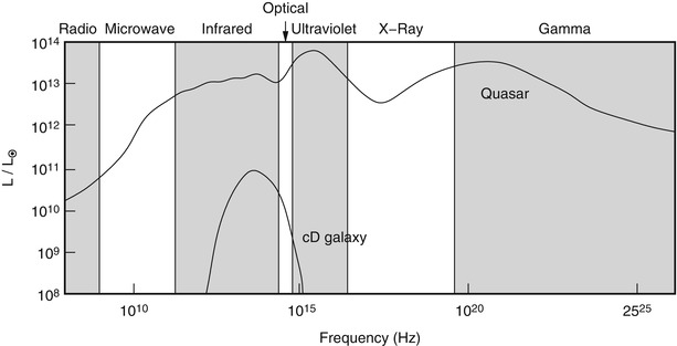
/epubstore/S/P-Schneider/Extragalactic-Astronomy-And-Cosmology/OEBPS/A129044_2_En_3_Fig4_HTML.jpg

Fig. 3.4

The spectrum of a quasar (3C273) in comparison to that of an elliptical galaxy, in terms of the ratio $\nu \,L_{\nu }/L_{\odot }$ . While the radiation from the elliptical is concentrated in a narrow range spanning less than two decades in frequency, the emission from the quasar is observed over the full range of the electromagnetic spectrum, and the energy per logarithmic frequency interval is roughly constant. This demonstrates that the light from the quasar cannot be interpreted as a superposition of stellar spectra, but instead has to be generated by completely different sources and by different radiation mechanisms

Besides the aforementioned main types of galaxy morphologies, others exist which do not fit into the Hubble scheme. Many of these are presumably caused by interaction between galaxies (see below). Furthermore, we observe galaxies with radiation characteristics that differ significantly from the spectral behavior of ‘normal’ galaxies. These galaxies will be discussed next.

3.1.2 Other types of galaxies

The light from ‘normal’ galaxies is emitted mainly by stars. Therefore, the spectral distribution of the radiation from such galaxies is in principle a superposition of the spectra of their stellar population. The spectrum of stars is, to a first approximation, described by a Planck function (see Appendix A) that depends only on the star’s surface temperature. A typical stellar population covers a temperature range from a few thousand Kelvin up to a few tens of thousand Kelvin. Since the Planck function has a well-localized maximum and from there steeply declines to both sides, most of the energy of such ‘normal’ galaxies is emitted in a relatively narrow frequency interval that is located in the optical and NIR sections of the spectrum.

In addition to these, other galaxies exist whose spectral distribution cannot be described by a superposition of stellar spectra. One example is the class of active galaxies which generate a significant fraction of their luminosity from gravitational energy that is released in the infall of matter onto a supermassive black hole, as was mentioned in Sect. 1.2.4. The activity of such objects can be recognized in various ways. For example, some of them are very luminous in the radio and/or in the X-ray portion of the spectrum (see Fig. 3.4), or they show strong emission lines with a width of several thousand km/s if the line width is interpreted as due to Doppler broadening, i.e., $\varDelta \lambda /\lambda =\varDelta v/c$ . In many cases, by far the largest fraction of luminosity is produced in a very small central region: the active galactic nucleus (AGN) that gave this class of galaxies its name. In quasars, the central luminosity can be of the order of ∼ 10¹³ L _⊙, about a thousand times as luminous as the total luminosity of our Milky Way. We will discuss active galaxies, their phenomena, and their physical properties in detail in Chap. 5

Another type of galaxy also has spectral properties that differ significantly from those of ‘normal’ galaxies, namely the starburst galaxies. Normal spiral galaxies like our Milky Way form new stars at a star-formation rate of ∼ 3M _⊙∕yr which can be derived, for instance, from the Balmer lines of hydrogen generated in the Hii regions around young, hot stars. By contrast, elliptical galaxies show only marginal star formation or none at all. However, there are galaxies which have a much higher star-formation rate, reaching values of 100M _⊙∕yr and more. If many young stars are formed we would expect these starburst galaxies to radiate strongly in the blue or in the UV part of the spectrum, corresponding to the maximum of the Planck function for the most massive and most luminous stars (see Fig. 3.5). This expectation is not fully met though: star formation takes place in the interior of dense molecular clouds which often also contain large amounts of dust. If the major part of star formation is hidden from our direct view by layers of absorbing dust, these galaxies will not be very prominent in blue light. However, the strong radiation from the young, luminous stars heats the dust; the absorbed stellar light is then re-emitted in the form of thermal dust emission in the infrared region of the electromagnetic spectrum—these galaxies can thus be extremely luminous in the IR. They are called ultra-luminous infrared galaxies (ULIRGs). We will describe the phenomena of starburst galaxies in more detail in Sect. 9.3.1. Of special interest is the discovery that the star-formation rate of galaxies seems to be closely related to interactions between galaxies—many ULIRGs are strongly interacting or merging galaxies (see Fig. 3.6).

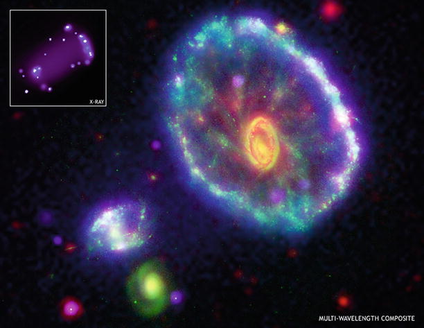
/epubstore/S/P-Schneider/Extragalactic-Astronomy-And-Cosmology/OEBPS/A129044_2_En_3_Fig5_HTML.jpg

Fig. 3.5

The Cartwheel galaxy is shown as a color composite, based on data with four different telescopes: the green color shows the optical light as seen with the HST, the red color shows the infrared emission as seen by Spitzer, in blue the ultraviolet emission as seen by GALEX is displayed, and purple shows the X-ray light observed with Chandra. This galaxy has a very unusual morphology, which is due to a collision with one of the smaller galaxies seen towards the lower left, some 200 million years ago. Before the collision it was probably a normal spiral galaxy, but the collision created a shock wave which swept up gas and formed a large ring, in which very active star formation started to occur. This intense star formation is seen clearly through its UV and X-ray emission, and some of the star-forming regions are also very luminous in the infrared. Many of the massive stars formed in this starburst exploded as supernovae, leaving behind neutrons stars and probably black holes. If these compact objects have a companion star, they can accrete matter and can become powerful X-ray sources, like the X-ray binaries seen in the Milky Way. We will see later that the triggering of starbursts through galaxy collisions is a very common phenomenon. Credit: Composite: NASA/JPL/Caltech/P.Appleton et al. X-ray: NASA/CXC/A. Wolter & G. Trinchieri et al.

Fig. 3.6

This mosaic of 9 HST images shows different ULIRGs in collisional interaction between two or more galaxies. Credit: NASA, STScI, K. Borne, L. Colina, H. Bushouse & R. Lucas

3.1.3 The bimodal color distribution of galaxies

The classification of galaxies by morphology, given by the Hubble classification scheme (Fig. 3.2), has the disadvantage that morphologies of galaxies are not easy to quantify. Traditionally, this was done by visual inspection but of course this method bears some subjectivity of the researcher doing it and requires a lot of experience. Furthermore, this visual inspection is time consuming and cannot be performed on large samples of galaxies. ² Various techniques and related software were developed to perform such a classification automatically, in many cases with significant success, including the reproducibility of galaxy classification between different methods. Nevertheless, quite a number of problems remain, such as the inclination dependence of the morphological appearance of a galaxy.

Even automatic classifications cannot be applied to galaxies for which the angular resolution of the imaging is not much better than the angular size of galaxies, that is, for distant objects. An alternative to morphological classification is provided by the colors of galaxies, which can be obtained from broad-band multi-color imaging. Colors are much easier to measure than morphology, in particular for very small galaxies. In addition, the physical properties of galaxies may be better characterized by their colors than by their morphology—the colors yield information about the stellar population, whereas the morphology is determined by the dynamics of the galaxy.

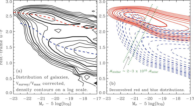
/epubstore/S/P-Schneider/Extragalactic-Astronomy-And-Cosmology/OEBPS/A129044_2_En_3_Fig7_HTML.jpg

Fig. 3.7

The density of galaxies in color-magnitude space. The color of ∼ 70 000 galaxies with redshifts 0. 01 ≤ z ≤ 0. 08 from the Sloan Digital Sky Survey is measured by the rest-frame u − r, i.e., after a (small) correction for their redshift was applied. The density contours, which were corrected for selection effects, are logarithmically spaced, with a factor of $\sqrt{ 2}$ between consecutive contours. (a) The measured distribution is shown. Obviously, two peaks of the galaxy density are clearly visible, one at a red color of u − r ∼ 2. 5 and an absolute magnitude of M _r ∼ −21, the other at a bluer color of u − r ∼ 1. 3 and significantly fainter magnitudes. (b) Corresponds to the modeled galaxy density, as is described in the text. Reused with permission from I.K. Baldry, M.L. Balogh, R. Bower, K. Glazebrook & R.C. Nichols 2004, Color bimodality: Implications for galaxy evolution, in: THE NEW COSMOLOGY: Conference on Strings and Cosmology, R. Allen (ed.), Conference Proceeding 743, p. 106, Fig. 1 (2004). ©2004, American Institute of Physics

Using photometric measurements and spectroscopy from the Sloan Digital Sky Survey (see Sect. 8.1.2), the colors and absolute magnitudes of low-redshift galaxies have been studied; their density distribution in a color-magnitude diagram is plotted in the left-hand side of Fig. 3.7. We see immediately that there are two density peaks of the galaxy distribution in this diagram: one at high luminosities and red color, the other at significantly fainter absolute magnitudes and much bluer color. It appears that the galaxies are distributed at and around these two density peaks, hence galaxies tend to be either luminous and red, or less luminous and blue. We can also easily see from this diagram that the distribution of red and blue galaxies with respect to their luminosity is different, the former one being more shifted towards larger luminosity.

We can next consider the color distribution of galaxies at a fixed absolute magnitude M _r . This is obtained by plotting the galaxy number density along vertical cuts through the left-hand side of Fig. 3.7. When this is done for different M _r , it turns out that the color distribution of galaxies is bimodal: over a broad range in absolute magnitude, the color distribution has two peaks, one at red, the other at blue u − r. Again, this fact can be seen directly from Fig. 3.7. For each value of M _r , the color distribution of galaxies can be very well fitted by the sum of two Gaussian functions. The central colors of the two Gaussians are shown by the two dashed curves in the left panel of Fig. 3.7. They become redder the more luminous the galaxies are. This luminosity-dependent reddening is considerably more pronounced for the blue population than for the red galaxies.

To see how good this fit indeed is, the right-hand side of Fig. 3.7 shows the galaxy density as obtained from the two-Gaussian fits, with solid contours corresponding to the red galaxies and dashed contours to the blue ones. We thus conclude that the local galaxy population can be described as a bimodal distribution in u − r color, where the characteristic color depends slightly on absolute magnitude. The galaxy distribution at bright absolute magnitudes is dominated by red galaxies, whereas for less luminous galaxies the blue population dominates.

The mass-to-light ratio of a red stellar population is larger than that of a blue population, since the former no longer contains massive luminous stars. The difference in the peak absolute magnitude between the red and blue galaxies therefore corresponds to an even larger difference in the stellar mass of these two populations. Red galaxies in the local Universe have on average a much higher stellar mass than blue galaxies. This fact is illustrated by the two dotted lines in the right-hand panel of Fig. 3.7 which correspond to lines of constant stellar mass of ∼ 2–3 × 10¹⁰ M _⊙. This seems to indicate a very characteristic mass scale for the galaxy distribution: most galaxies with a stellar mass larger than this characteristic mass scale are red, whereas most of those with a lower stellar mass are blue.

Obviously, these statistical properties of the galaxy distribution must have an explanation in terms of the evolution of galaxies; we will come back to this issue in Chap. 9. Furthermore, in Sect. 3.6 we will relate the morphological classification to that in color-magnitude space. But first we will describe the properties of elliptical and spiral galaxies in more detail in the next two sections.

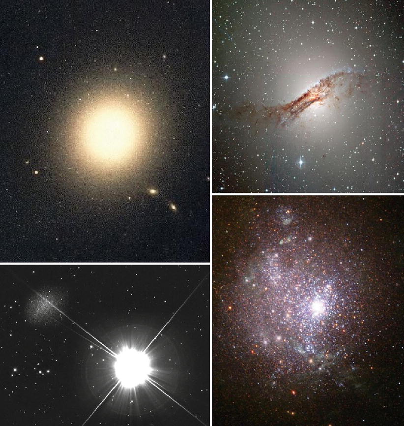
/epubstore/S/P-Schneider/Extragalactic-Astronomy-And-Cosmology/OEBPS/A129044_2_En_3_Fig8_HTML.jpg

Fig. 3.8

Different types of elliptical galaxies. Upper left: the cD galaxy M87 in the center of the Virgo galaxy cluster; upper right: Centaurus A, a giant elliptical galaxy with a very distinct dust disk and an active galactic nucleus; lower left: the galaxy Leo I (located near the upper left corner of the image) belongs to the nine known dwarf spheroidals in the Local Group; lower right: NGC 1705, a dwarf irregular, shows indications of massive star formation—a super star cluster and strong galactic winds. Credit: Top left: Digital Sky Survey, ESO. Top right: ESO. Bottom left: Michael Breite, www.skyphoto.de. Bottom right: NASA, ESA and The Hubble Heritage Team (STScI/AURA); acknowledgement: M. Tosi (INAF, Osservatorio Astronomico di Bologna)

Table 3.1

Characteristic values for early-type galaxies

	S0	cD	E	dE	dSph	BCD
M _B	−17 to −22	−22 to −25	−15 to −23	−13 to −19	−8 to −15	−14 to −17
M (M_⊙)	10¹⁰–10¹²	10¹³–10¹⁴	10⁸–10¹³	10⁷–10⁹	10⁷–10⁸	∼ 10⁹
D ₂₅ (kpc)	10–100	300–1000	1–200	1–10	0.1–0.5	< 3
$\langle M/L_{\mathrm{B}}\rangle$	∼ 10	> 100	10–100	1–10	5–100	0.1–10
$\langle S_{\mathrm{N}}\rangle$	∼ 5	∼ 15	∼ 5	4.8 ± 1.0	–	–

D ₂₅ denotes the diameter at which the surface brightness has decreased to 25 B-mag/arcsec², S _N is the ‘specific frequency’, a measure for the number of globular clusters in relation to the visual luminosity [see (3.18)], and M∕L is the mass-to-light ratio in Solar units (the values of this table are taken from the book by Carroll & Ostlie)

3.2 Elliptical Galaxies

3.2.1 Classification

The general term ‘elliptical galaxies’ (or ellipticals, for short) covers a broad class of galaxies which differ in their luminosities and sizes—some of them are displayed in Fig. 3.8. A rough subdivision is as follows:

Normal ellipticals. This class includes giant ellipticals (gE’s), those of intermediate luminosity (E’s), and compact ellipticals (cE’s), covering a range in absolute magnitudes from M _B ∼ −23 to M _B ∼ −15.
Dwarf ellipticals (dE’s). These differ from the cE’s in that they have a significantly smaller surface brightness and a lower metallicity.
cD galaxies . These are extremely luminous (up to M _B ∼ −25) and large (up to $R \lesssim 1\,\mathrm{Mpc}$ ) galaxies that are only found near the centers of dense clusters of galaxies. Their surface brightness is very high close to the center, they have an extended diffuse envelope, and they have a very high M∕L ratio. As we will discuss in Sect. 6.3.4, it is not clear whether the extended envelope actually ‘belongs’ to the galaxy or is part of the galaxy cluster in which the cD is embedded, since such clusters are now known to have a population of stars located outside of the cluster galaxies.
Blue compact dwarf galaxies. These ‘blue compact dwarfs’ (BCD’s) are clearly bluer (with $\left \langle B - V \right \rangle$ between 0.0 and 0.3) than the other ellipticals, and contain an appreciable amount of gas in comparison.
Dwarf spheroidals (dSph’s) exhibit a very low luminosity and surface brightness. They have been observed down to M _B ∼ −8. Due to these properties, they have thus far only been observed in the Local Group.

Thus elliptical galaxies span an enormous range (more than 10⁶) in luminosity and mass, as is shown by the compilation in Table 3.1.

3.2.2 Brightness profile

The brightness profiles of normal E’s and cD’s follow approximately a de Vaucouleurs profile [see (2.40) or (2.42), respectively] over a wide range in radius, as is illustrated in Fig. 3.9. The effective radius R _e is strongly correlated with the absolute magnitude M _B , as can be seen in Fig. 3.10, with rather little scatter. In comparison, the dE’s and the dSph’s clearly follow a different distribution. Owing to the relation (2.43) between luminosity, effective radius and central surface brightness, an analogous relation exists for the average surface brightness μ _ave (unit: B-mag/arcsec²) within R _e as a function of M _B . In particular, the surface brightness in normal E’s decreases with increasing luminosity, while it increases for dE’s and dSph’s.

Yet another way of expressing this correlation is by eliminating the absolute luminosity, obtaining a relation between effective radius R _e and surface brightness μ _avg. This form is then called the Kormendy relation.

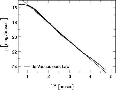
/epubstore/S/P-Schneider/Extragalactic-Astronomy-And-Cosmology/OEBPS/A129044_2_En_3_Fig9_HTML.jpg

Fig. 3.9

Surface brightness profile of the galaxy NGC 4472, fitted by a de Vaucouleurs profile (solid curve). The de Vaucouleurs profile describes a linear relation between the logarithm of the intensity (i.e., linear on a magnitude scale) and r ^1∕4; for this reason, it is also called an r ^1∕4-law

The de Vaucouleurs profile provides good fits for normal E’s, whereas for E’s with exceptionally high (or low) luminosity the profile decreases more slowly (or rapidly) for larger radii. The profile of cD’s extends much farther out and is not properly described by a de Vaucouleurs profile (Fig. 3.11), except in it innermost part. It appears that cD’s are similar to E’s but embedded in a very extended, luminous halo. Since cD’s are only found in the centers of massive clusters of galaxies, a connection must exist between this morphology and the environment of these galaxies; we shall return to this topic in Sect. 6.3.4. In contrast to these classes of ellipticals, diffuse dE’s are often better described by an exponential profile. In fact, the large recent surveys allowed a much better characterization of the brightness profiles of ellipticals and variations amongst them, as will be discussed in Sect. 3.6.

Cores and extra light. As indicated in Fig. 3.9, the brightness profile can differ significantly from a de Vaucouleurs profile in the very central part; in the example shown, the central brightness profile lies well below the r ^1∕4 fit. In this case, the central brightness profile is said to have a core , or a light deficit (relative to the extrapolation of the de Vaucouleurs profile towards the center). Ellipticals with a core are typically very luminous (and correspondingly have a high stellar mass). Also the opposite effect occurs: some ellipticals, typically those of lower luminosity, have an excess of light in their cores, relative to the extrapolation of the brightness profile fit at larger radii.

3.2.3 Composition of elliptical galaxies

Except for the BCD’s, elliptical galaxies appear red when observed in the optical, which suggests an old stellar population. It was once believed that ellipticals contain neither gas nor dust, but these components have now been found, though at a much lower mass-fraction than in spirals. For example, in some ellipticals hot gas ( ∼ 10⁷K) is detected by its X-ray emission. Furthermore, Hα emission lines of warm gas ( ∼ 10⁴ K) are observed, as well as cold gas ( ∼ 100 K) in the Hi (21 cm) and CO molecular lines. Many (up to 75 % of the population) of the normal ellipticals contain visible amounts of dust, partially manifested as a dust disk (see the upper right panel of Fig. 3.8 for a prominent example). They frequently show extended Hi disks, up to ∼ 200 kpc in diameter. However, the estimated mass of the cold atomic and molecular gas is typically less than 1 % of the stellar mass in ellipticals. This amount of gas is actually smaller than expected from the gas release from the stellar population due to its evolution, e.g., in the form of stellar winds, planetary nebulae etc. The fate of the bulk of this gas is currently unclear.

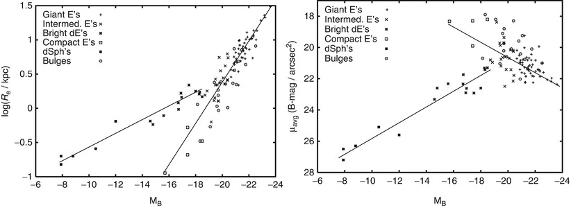
/epubstore/S/P-Schneider/Extragalactic-Astronomy-And-Cosmology/OEBPS/A129044_2_En_3_Fig10_HTML.jpg

Fig. 3.10

Left panel: effective radius R _e versus absolute magnitude M _B ; the correlation for normal ellipticals is different from that of dwarfs. Right panel: average surface brightness μ _avg versus M _B ; with increasing luminosity, the surface brightness of normal ellipticals decreases, while for dwarf ellipticals and spheroidals it increases. Source: R. Bender et al. 1992, Dynamically hot galaxies. I - Structural properties, ApJ 399, 462. ©AAS. Reproduced with permission

Whereas the largest fraction of the stellar population in ellipticals is old—as we will see soon, most of the stars in present-day ellipticals must have formed some 10 billion years ago—there are spectroscopic indications for a low level of recent star formation. This has been further supported from UV-observations carried out by the GALEX satellite which showed that ∼ 15 % of galaxies which are red in optical colors (and thus located in the upper peak of the color-magnitude diagram in Fig. 3.7) show a strong UV-excess. Spatially resolved imaging of early-type galaxies with an UV-excess at wavelengths of $\lambda \sim 1500\,\mathrm{{\AA}}$ showed that about 75 % of them do indeed clearly display star-formation activity (see Fig. 3.12 for four examples). The UV emission is more extended that the optical image of the galaxies, i.e., the star formation occurs in the outer parts of the galaxies. The star-formation rate is sufficiently low ( ∼ 0. 5M _⊙∕yr) as to have a vanishing effect on the optical colors of these galaxies. The large radii at which the UV emission is seen suggests that the stars do not form from gas which has been located in the gravitational potential of the galaxy; instead, it is likely that it is gas infalling from the surrounding medium. We have seen direct evidence for such infalling gas in the Milky Way (see Sect. 2.3.7), and in Chap. 10 we will explain that such gas infall is indeed expected in our model of structure formation in the Universe.

/epubstore/S/P-Schneider/Extragalactic-Astronomy-And-Cosmology/OEBPS/A129044_2_En_3_Fig11_HTML.jpg

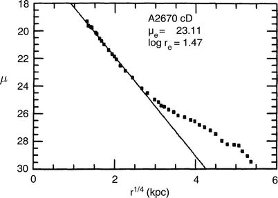
Fig. 3.11

Comparison of the brightness profile of a cD galaxy, the central galaxy of the cluster of galaxies Abell 2670, with a de Vaucouleurs profile. The light excess for large radii is clearly visible. Source: J.M. Schombert 1986, The structure of brightest cluster members. I - Surface photometry, ApJS 60, 603, p. 618, Fig. 1. ©AAS. Reproduced with permission

The metallicity of ellipticals and S0 galaxies increases towards the galaxy center, as derived from color gradients. Also in S0 galaxies the bulge appears redder than the disk. The Spitzer Space Telescope, launched in 2003, detected a spatially extended distribution of warm dust in S0 galaxies, organized in some sort of spiral structure. Cold dust was also found in ellipticals and S0 galaxies.

This composition of ellipticals clearly differs from that of spiral galaxies and needs to be explained by models of the formation and evolution of galaxies. We will see later that the cosmic evolution of elliptical galaxies is also observed to be different from that of spirals.

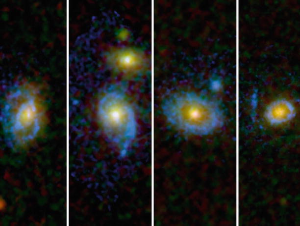
/epubstore/S/P-Schneider/Extragalactic-Astronomy-And-Cosmology/OEBPS/A129044_2_En_3_Fig12_HTML.jpg

Fig. 3.12

Four early-type galaxies, observed at UV and optical wavelengths with HST. The optical emission is shown in green, yellow and red, whereas the UV emission is shown in blue. Credit: NASA/ESA/JPL-Caltech/STScI/UCLA

3.2.4 Dynamics of elliptical galaxies

Analyzing the morphology of elliptical galaxies raises a simple question: Why are ellipticals not round? A simple explanation would be rotational flattening, i.e., as in a rotating self-gravitating gas ball, the stellar distribution bulges outwards at the equator due to centrifugal forces, as is also the case for the Earth. If this explanation was correct, the rotational velocity v _rot, which is measurable in the relative Doppler shift of absorption lines, would have to be of about the same magnitude as the velocity dispersion of the stars σ _v that is measurable through the Doppler broadening of lines. More precisely, by means of stellar dynamics one can show that for the rotational flattening of an axially symmetric, oblate³ galaxy, the relation

$\displaystyle{ \left (\frac{v_{\mathrm{rot}}} {\sigma _{v}} \right )_{\mathrm{iso}} \approx \sqrt{ \frac{\epsilon } {1 -\epsilon }} }$

(3.1)

has to be satisfied, where ‘iso’ indicates the assumption of an isotropic velocity distribution of the stars. However, for very luminous ellipticals one finds that, in general, v _rot ≪ σ _v , so that rotation cannot be the major cause of their ellipticity (see Fig. 3.13). In addition, many ellipticals are presumably triaxial, so that no unambiguous rotation axis is defined. Thus, luminous ellipticals are in general not rotationally flattened. For less luminous ellipticals and for the bulges of disk galaxies, however, rotational flattening can play an important role. The question remains of how to explain a stable elliptical distribution of stars without bulk rotation.

/epubstore/S/P-Schneider/Extragalactic-Astronomy-And-Cosmology/OEBPS/A129044_2_En_3_Fig13_HTML.jpg

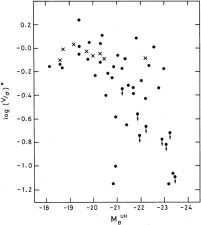
Fig. 3.13

The rotation parameter $\left (\frac{v_{\mathrm{rot}}} {\sigma _{v}} \right )/\left (\frac{v_{\mathrm{rot}}} {\sigma _{v}} \right )_{\mathrm{iso}}$ of elliptical galaxies, here denoted by (V/σ)^∗, plotted as a function of absolute magnitude. Dots denote elliptical galaxies, crosses the bulges of disk galaxies; arrows indicate that the corresponding dot is an upper limit on the rotation parameter. One sees that the luminous ellipticals rotate far too slow to explain their ellipticity as being due to rotational flattening, whereas lower-luminosity objects can be rotationally flattened. Source: R.L. Davies et al. 1983, The kinematic properties of faint elliptical galaxies, ApJ 266, 41, p. 49, Fig. 4. ©AAS. Reproduced with permission

The brightness profile of an elliptical galaxy is defined by the distribution of its stellar orbits. Let us assume that the gravitational potential is given. The stars are then placed into this potential, with the initial positions and velocities following a specified distribution. If this distribution is not isotropic in velocity space, the resulting light distribution will in general not be spherical. For instance, one could imagine that the orbital planes of the stars have a preferred direction, but that an equal number of stars exists with positive and negative angular momentum L _z , so that the total stellar distribution has no net angular momentum and therefore does not rotate. Each star moves along its orbit in the gravitational potential, where the orbits are in general not closed. If an initial distribution of stellar orbits is chosen such that the statistical properties of the distribution of the orbits are invariant in time, then one will obtain a stationary system. If, in addition, the distribution is chosen such that the respective mass distribution of the stars will generate exactly the originally chosen gravitational potential, one arrives at a self-gravitating equilibrium system. In general, it is a difficult mathematical problem to construct such self-gravitating equilibrium systems. Furthermore, as we will see, elliptical galaxies also contain a dark matter component, whose gravitational potential adds to that of the stars.

Relaxation time-scale. The question now arises whether such an equilibrium system can also be stable in time. One might expect that close encounters of pairs of stars would cause a noticeable disturbance in the distribution of orbits. These pair-wise collisions could then lead to a ‘thermalization’ of the stellar orbits.⁴ To examine this question we need to estimate the time-scale for such collisions and the changes in direction they cause.

For this purpose, we consider the relaxation time-scale by pair collisions in a system of N stars of mass m, total mass M = Nm, extent R, and a mean stellar density of $n = 3N/(4\pi R^{3})$ . We define the relaxation time t _relax as the characteristic time in which a star changes its velocity direction by ∼ 90^∘ due to pair collisions with other stars. By simple calculation (see below), we find that

$\displaystyle{ t_{\mathrm{relax}} \approx \frac{R} {6v} \frac{N} {\ln (N/2)}\;, }$

(3.2)

$\displaystyle{ \fbox{$t_{\mathrm{relax}} = \frac{t_{\mathrm{cross}}} {6} \frac{N} {\ln (N/2)}$}\;, }$

(3.3)

where $t_{\mathrm{cross}} = R/v$ is the crossing time-scale, i.e. the time it takes a star to cross the stellar system. If we now consider a typical galaxy, with $t_{\mathrm{cross}} \sim 10^{8}\,\mathrm{yr}$ , N ∼ 10¹² [thus ln(N∕2) ∼ 30], then we find that the relaxation time is much longer than the age of the Universe. This means that pair collisions do not play any role in the evolution of stellar orbits. The dynamics of the orbits are determined solely by the large-scale gravitational field of the galaxy. In Sect. 7.5.1, we will describe a process called violent relaxation which most likely plays a central role in the formation of galaxies and which is probably also responsible for the stellar orbits establishing an equilibrium configuration.

We thus conclude that the stars behave like a collisionless gas: elliptical galaxies are stabilized by (dynamical) pressure, and they are elliptical because the stellar distribution is anisotropic in velocity space. This corresponds to an anisotropic pressure—where we recall that the pressure of a gas is nothing but the momentum transport of gas particles due to their thermal motion.

Derivation of the collisional relaxation time-scale. We consider a star passing by another one, with the impact parameter b being the minimum distance between the two. From gravitational deflection, the star attains a velocity component perpendicular to the incoming direction of

$\displaystyle{ \fbox{$v_{\perp }^{(1)} \approx a\,\varDelta t \approx \left (\frac{\mathit{Gm}} {b^{2}} \right )\left (\frac{2b} {v} \right ) = \frac{2\mathit{Gm}} {bv} $}\;, }$

(3.4)

where a is the acceleration at closest separation and Δ t the ‘duration of the collision’, estimated as $\varDelta t = 2b/v$ (see Fig. 3.14). Equation (3.4) can be derived more rigorously by integrating the perpendicular acceleration along the orbit. A star undergoes many collisions, through which the perpendicular velocity components will accumulate; these form two-dimensional vectors perpendicular to the original direction. After a time t we have ${\boldsymbol v}_{\perp }(t) =\sum _{i}{\boldsymbol v}_{\perp }^{(i)}$ . The expectation value of this vector is $\left \langle {\boldsymbol v}_{\perp }(t)\right \rangle =\sum _{i}\left \langle {\boldsymbol v}_{\perp }^{(i)}\right \rangle = 0$ since the directions of the individual ${\boldsymbol v}_{\perp }^{(i)}$ are random. But the mean square velocity perpendicular to the incoming direction does not vanish,

$\displaystyle{ \left \langle \left \vert {\boldsymbol v}_{\perp }\right \vert ^{2}(t)\right \rangle =\sum _{ ij}\left \langle {\boldsymbol v}_{\perp }^{(i)} \cdot {\boldsymbol v}_{ \perp }^{(j)}\right \rangle =\sum _{ i}\left \langle \left \vert {\boldsymbol v}_{\perp }^{(i)}\right \vert ^{2}\right \rangle \neq 0\;, }$

(3.5)

where we set $\left \langle {\boldsymbol v}_{\perp }^{(i)} \cdot {\boldsymbol v}_{\perp }^{(j)}\right \rangle = 0$ for i ≠ j because the directions of different collisions are assumed to be uncorrelated. The velocity ${\boldsymbol v}_{\perp }$ performs a so-called random walk. To compute the sum, we convert it into an integral where we have to integrate over all collision parameters b. During time t, all collision partners with impact parameters within db of b are located in a cylindrical shell of volume (2π b db) (vt), so that

$\displaystyle\begin{array}{rcl} \left \langle \left \vert {\boldsymbol v}_{\perp }\right \vert ^{2}(t)\right \rangle & =& \int 2\pi \,b\,\mathrm{d}b\,v\,t\;n\;\left \vert v_{ \perp }^{(1)}\right \vert ^{2} \\ & =& 2\pi \left (\frac{2\mathit{Gm}} {v} \right )^{2}v\,t\,n\int \frac{\mathrm{d}b} {b} \;.{}\end{array}$

(3.6)

The integral cannot be performed from 0 to ∞. Thus, it has to be cut off at b _min and b _max and then yields $\ln (b_{\mathrm{max}}/b_{\mathrm{min}})$ . Due to the finite size of the stellar distribution, b _max = R is a natural choice. Furthermore, our approximation which led to (3.4) will certainly break down if $v_{\perp }^{(1)}$ is of the same order of magnitude as v; hence we choose $b_{\mathrm{min}} = 2\mathit{Gm}/v^{2}$ . With this, we obtain $b_{\mathrm{max}}/b_{\mathrm{min}} = Rv^{2}/(2\mathit{Gm})$ . The exact choice of the integration limits is not important, since b _min and b _max appear only logarithmically. Next, using the virial theorem, $\left \vert E_{\mathrm{pot}}\right \vert = 2E_{\mathrm{kin}}$ , and thus $\mathit{GM}/R = v^{2}$ for a typical star, we get $b_{\mathrm{max}}/b_{\mathrm{min}} \approx N/2$ . Thus,

$\displaystyle{ \fbox{$\left \langle \left \vert {\boldsymbol v}_{\perp }\right \vert ^{2}(t)\right \rangle = 2\pi \left (\frac{2\mathit{Gm}} {v} \right )^{2}v\,t\,n\,\ln (N/2)$}\;. }$

(3.7)

We define the relaxation time t _relax by $\left \langle \left \vert {\boldsymbol v}_{\perp }\right \vert ^{2}(t_{\mathrm{relax}})\right \rangle = v^{2}$ , i.e., the time after which the perpendicular velocity roughly equals the infall velocity:

$\displaystyle\begin{array}{rcl} t_{\mathrm{relax}}& =& \frac{1} {2\pi nv}\left ( \frac{v^{2}} {2\mathit{Gm}}\right )^{2} \frac{1} {\ln (N/2)} \\ & =& \frac{1} {2\pi nv}\left ( \frac{M} {2\mathit{Rm}}\right )^{2} \frac{1} {\ln (N/2)} = \frac{R} {6v} \frac{N} {\ln (N/2)}\;,\quad {}\end{array}$

(3.8)

from which we finally obtain (3.3).

Fig. 3.14

Sketch related to the derivation of the dynamical time-scale

The Jeans equation. The behavior of stars in an elliptical galaxy is thus that of collisionless particles in a gravitational potential. The equation governing the density of stars as a function of position, velocity, and time, i.e., the phase-space density $f({\boldsymbol r},{\boldsymbol v},t)$ , is the collisionless Boltzmann equation. Without going into any detail, we shall quote one special result from the Boltzmann equation, which applies to the simplest case: Consider a spherically symmetric gravitational potential Φ(r), in which stars are orbiting. We assume that the system is stationary, so that the phase-space density f does not depend on time. Furthermore, the system is assumed to have no net rotation. The stellar distribution is assumed to be spherically symmetric as well, and the velocity distribution in the plane perpendicular to the radius vector should be isotropic. In spherical coordinates, this means that the velocity dispersion in the θ-direction is the same as that in the φ-direction, $\left \langle v_{\theta }^{2}\right \rangle = \left \langle v_{\varphi }^{2}\right \rangle$ . However, the velocity dispersion $\left \langle v_{r}^{2}\right \rangle$ in the radial direction is allowed to be different from that in the tangential direction. We quantify the anisotropy of the velocity distribution by the parameter

$\displaystyle{ \beta = 1 - \frac{\left \langle v_{\theta }^{2}\right \rangle } {\left \langle v_{r}^{2}\right \rangle }\;. }$

(3.9)

For example, if all stars would be on circular orbits, then $\left \langle v_{r}^{2}\right \rangle = 0$ , corresponding to $\beta = -\infty$ . Conversely, in the case that all stars are on radial orbits, one has β = 1. If the velocity distribution is isotropic, then β = 0. From the collisionless Boltzmann equation, one obtains the Jeans equation

$\displaystyle{ \frac{1} {n}\,\frac{\mathrm{d}\left (n\left \langle v_{r}^{2}\right \rangle \right )} {\mathrm{d}r} + 2\frac{\beta \left \langle v_{r}^{2}\right \rangle } {r} = -\frac{\mathrm{d}\varPhi } {\mathrm{d}r}\;, }$

(3.10)

relating the local volume density of particles

$\displaystyle{n(r) =\int \mathrm{ d}^{3}v\;f(x,{\boldsymbol v})\;,}$

and the velocity distribution characterized by $\left \langle v_{r}^{2}\right \rangle (r)$ and β(r) to the gravitational potential Φ(r).

Suppose we can measure the density of stars n(r), by mapping the surface brightness of an elliptical galaxy, assuming a mean stellar luminosity (which then yields the column density of stars, i.e., the projected stellar number density), and calculating n(r) from the projected density; for spherically symmetric distributions, these two are uniquely related to each other. Furthermore, suppose we obtain the line-of-sight velocity dispersion as a function of projected radius from spectroscopically determining the width of stellar absorption lines. This measured line-of-sight velocity dispersion depends on n(r), $\left \langle v_{r}^{2}\right \rangle (r)$ and the anisotropy parameter β(r). With n(r) determined from the projected number density, the observed velocity dispersion then depends on the two functions $\left \langle v_{r}^{2}\right \rangle (r)$ and β(r). Thus, the latter two cannot be determined separately from measurements of the observed line-of-sight velocity dispersion. This has an immediate consequence for the determination of the mass profile: let $\varPhi (r) = -\mathit{GM}(r)/r$ , then the mass profile of the galaxy is described by

$\displaystyle\begin{array}{rcl} v_{\mathrm{c}}^{2}(r) \equiv \frac{\mathit{GM}(r)} {r} = -\left \langle v_{r}^{2}\right \rangle \left (\frac{\mathrm{d}\ln n} {\mathrm{d}\ln r} + \frac{\mathrm{d}\ln \left \langle v_{r}^{2}\right \rangle } {\mathrm{d}\ln r} + 2\beta \right )\;,& &{}\end{array}$

(3.11)

where v _c(r) is the velocity that a particle on a circular orbit with radius r has in this potential. Since β and $\left \langle v_{r}^{2}\right \rangle$ cannot be determined separately, the mass profile of the galaxy cannot be measured. Or phrased differently, the mass estimate depends on the assumed anisotropy of the stellar orbits, so that mass profile and anisotropy are degenerate.

Therefore, even in the simplest case of maximum symmetry, the determination of the mass profile of elliptical galaxies is problematic. This is the reason why it is much more difficult to make accurate statements about the mass of ellipticals as obtained from stellar kinematics than it is for spiral galaxies, where the rotation curve yields the mass profile directly. Breaking the degeneracy between the radial velocity dispersion and the anisotropy parameter is possible, however, if one studies not only the line width of the stellar absorption lines, but also their shape. This shape depends on higher-order moments of the velocity distribution, and can be used to estimate $\left \langle v_{r}^{2}\right \rangle (r)$ and β(r) separately.

3.2.5 Indicators of a complex evolution

The isophotes (that is, the curves of constant surface brightness) of many of the normal elliptical galaxies are well approximated by ellipses. These elliptical isophotes with different surface brightnesses are concentric to high accuracy, with the deviation of the isophote’s center from the center of the galaxy being typically ≲ 1 % of its extent. However, in many cases the ellipticity varies with radius, so that the value for ε is not a constant. In addition, a few percent of ellipticals show a so-called isophote twist: the orientation of the semi-major axis of the isophotes changes with the surface brightness, and thus with radius. This indicates that elliptical galaxies are not spheroidal, but triaxial systems (or that there is some intrinsic twist of their axes).

Although the light distribution of ellipticals appears rather simple at first glance, a more thorough analysis reveals that the kinematics can be quite complicated. For example, dust disks are not necessarily perpendicular to any of the principal axes, and the dust disk may rotate in a direction opposite to the galactic rotation. In addition, ellipticals may also contain (weak) stellar disks.

Boxiness and diskiness. The so-called boxiness parameter describes the deviation of the isophotes’ shape from that of an ellipse. Consider the shape of an isophote. If it is described by an ellipse, then after a suitable choice of the coordinate system, θ ₁ = acost, θ ₂ = bsint, where a and b are the two semi-axes of the ellipse and t ∈ [0, 2π] parametrizes the curve. The distance r(t) of a point from the center is

$\displaystyle{r(t) = \sqrt{\theta _{1 }^{2 } +\theta _{ 2 }^{2}} = \sqrt{\frac{a^{2 } + b^{2 } } {2} + \frac{a^{2} - b^{2}} {2} \,\cos (2t)}\;.}$

Deviations of the isophote shape from this ellipse are now expanded in a Taylor series, where the term $\propto \cos (4t)$ describes the lowest-order correction that preserves the symmetry of the ellipse with respect to reflection in the two coordinate axes. The modified curve is then described by

$\displaystyle{ {\boldsymbol \theta }(t) = \left (1 + \frac{a_{4}\,\cos (4t)} {r(t)} \right )\left (\begin{array}{c} a\cos t\\ b\sin t\end{array} \right )\;, }$

(3.12)

with r(t) as defined above. The parameter a ₄ thus describes a deviation from an ellipse: if a ₄ > 0, the isophote appears more disk-like, and if a ₄ < 0, it becomes rather boxy (see Fig. 3.15). In most elliptical galaxies we typically find $\left \vert a_{4}/a\right \vert \sim 0.01$ , thus only a small deviation from the elliptical form.

/epubstore/S/P-Schneider/Extragalactic-Astronomy-And-Cosmology/OEBPS/A129044_2_En_3_Fig15_HTML.jpg

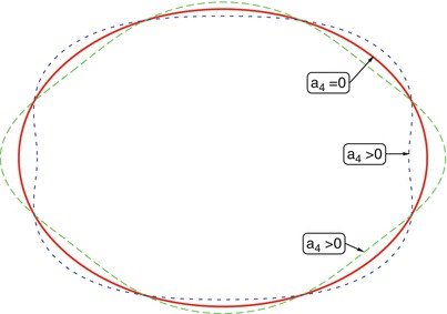
Fig. 3.15

Sketch to illustrate boxiness and diskiness. The solid red curve shows an ellipse (a ₄ = 0), the green dashed curve a disky ellipse (a ₄ > 0), and the blue dotted curve a boxy ellipse (a ₄ < 0). In most elliptical galaxies, the deviations in the shape of the isophotes from an ellipse are considerably smaller than in this sketch

Correlations of a ₄ with other properties of ellipticals. At first sight, such apparently small deviations from an exact elliptical shape of isophotes seems to be of little importance. Surprisingly however, we find that the parameter a ₄∕a is strongly correlated with other properties of ellipticals (see Fig. 3.16). The ratio $\left (\frac{v_{\mathrm{rot}}} {\sigma _{v}} \right )/\left (\frac{v_{\mathrm{rot}}} {\sigma _{v}} \right )_{\mathrm{iso}}$ (upper left in Fig. 3.16) is of order unity for disky ellipses (a ₄ > 0) and, in general, significantly smaller than one for boxy ellipticals. From this we conclude that ‘diskies’ are in part rotationally supported, whereas the flattening of ‘boxies’ is mainly caused by the anisotropic distribution of their stellar orbits in velocity space. The mass-to-light ratio is also correlated with a ₄: boxies (diskies) have a value of M∕L in their core which is larger (smaller) than the mean elliptical of comparable luminosity. A very strong correlation exists between a ₄∕a and the radio luminosity of ellipticals: while diskies are weak radio emitters, boxies show a broad distribution in L _radio. These correlations are also seen in the X-ray luminosity, since diskies are weak X-ray emitters and boxies have a broad distribution in L _X. This bimodality becomes even more obvious if the radiation contributed by compact sources (e.g., X-ray binary stars) is subtracted from the total X-ray luminosity, thus considering only the diffuse X-ray emission. Ellipticals with a different sign of a ₄ also differ in the kinematics of their stars: boxies often have cores spinning against the general direction of rotation (counter-rotating cores), which is rarely observed in diskies.

About 70 % of the ellipticals are diskies. The transition between diskies and S0 galaxies may be continuous along a sequence of varying disk-to-bulge ratio.

Fig. 3.16

Correlations of a ₄∕a with some other properties of elliptical galaxies. 100a(4)∕a (corresponding to a ₄∕a) describes the deviation of the isophote shape from an ellipse in percent. Negative values denote boxy ellipticals, positive values disky ellipticals. The upper left panel shows the rotation parameter discussed in Sect. 3.2.4; at the lower left, the deviation from the average mass-to-light ratio is shown. The upper right panel shows the ellipticity, and the lower right panel displays the radio luminosity at 1.4 GHz. Obviously, there is a correlation of all these parameters with the boxiness parameter. Source: J. Kormendy & S. Djorgovski 1989, Surface photometry and the structure of elliptical galaxies, ARA&A 27, 235, Fig. 3, p. 259. Reprinted, with permission, from the Annual Review of Astronomy & Astrophysics, Volume 27 ©1989 by Annual Reviews www.annualreviews.org

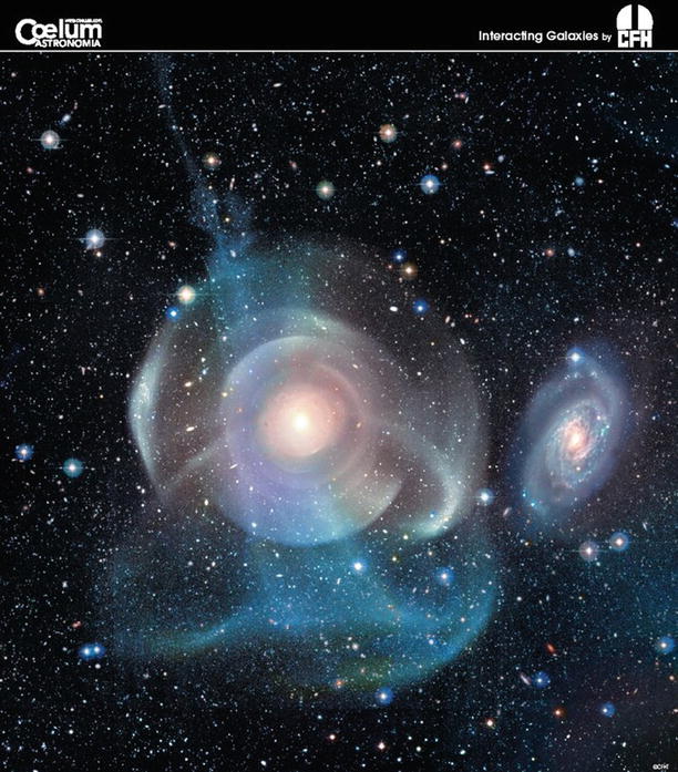
/epubstore/S/P-Schneider/Extragalactic-Astronomy-And-Cosmology/OEBPS/A129044_2_En_3_Fig17_HTML.jpg

Fig. 3.17

As a result of galaxy collisions and mergers, coherent stellar structures are formed, as seen in the galaxy NGC 474, one of the most spectacular examples found so far. The galaxy has multiple luminous shells and a complex structure of tidal tails, witnesses of its past violent history. Credit: Jean-Charles Cuillandre (CFHT) & Giovanni Anselmi (Coelum)/Canada-France-Hawaii Telescope/Coelum

Shells and ripples. In many of the early-type galaxies that are not member galaxies of a cluster, sharp discontinuities in the surface brightness are found, a kind of shell structure (‘shells’ or ‘ripples’). They are visible as elliptical arcs curving around the center of the galaxy (see Fig. 3.17). Such sharp edges can only be formed if the corresponding distribution of stars is ‘cold’, i.e., they must have a very small velocity dispersion, since otherwise such coherent structures would smear out on a very short time-scale. As a comparison, we can consider disk galaxies that likewise contain sharp structures, namely the thin stellar disk. Indeed, the stars in the disk have a very small velocity dispersion, ∼ 20 km∕s, compared to the rotational velocity of typically 200 km∕s. Probably a better example are the stellar streams discovered in the halo of the Milky Way (Sect. 2.3.6) which remain coherent through orbiting the Galaxy only because the velocity dispersion of stars belonging to these streams is much smaller than the characteristic rotational velocity.

These peculiarities in ellipticals are not uncommon. Indicators for shells and other tidal features can be found in about 70 % of the early-type galaxies, and about a third of them show boxy isophotes.

Boxiness, counter-rotating cores, and shells and ripples are all indicators of a complex evolution that is probably caused by past interactions and mergers with other galaxies.

We will proceed with a discussion of this interpretation in Chap. 10.

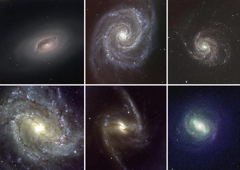
/epubstore/S/P-Schneider/Extragalactic-Astronomy-And-Cosmology/OEBPS/A129044_2_En_3_Fig18_HTML.jpg

Fig. 3.18

Types of spiral galaxies. Top left: M94, an Sab galaxy. Top middle: M51, an Sbc galaxy. Top right: M101, an Sc galaxy. Lower left: M83, an SBa galaxy. Lower middle: NGC 1365, an SBb galaxy. Lower right: M58, an SBc galaxy. Credit: Top left: Jacobus Kapteyn Telescope, ING Archive and Nik Szymanek. Top middle: William Herschel Telescope, ING Archive, Javier Méndez and Nik Szymanek. Top right: INT, Peter Bunclark and Nik Szymanek. Lower left: European Southern Observatory. Lower middle: European Southern Observatory. Lower right: JKT, Johan Knapen and Nik Szymanek

3.3 Spiral galaxies

3.3.1 Trends in the sequence of spirals

Looking at the sequence of early-type spirals (i.e., Sa’s or SBa’s) to late-type spirals, we find a number of differences that can be used for classification (see Fig. 3.18):

a decreasing luminosity ratio of bulge and disk, with $L_{\mathrm{bulge}}/L_{\mathrm{disk}} \sim 0.3$ for Sa’s and ∼ 0. 05 for Sc’s,
an increasing opening angle of the spiral arms, from ∼ 6^∘ for Sa’s to ∼ 18^∘ for Sc’s,
and an increasing brightness structure along the spiral arms: Sa’s have a ‘smooth’ distribution of stars along the spiral arms, whereas the light distribution in the spiral arms of Sc’s is resolved into bright knots of stars and Hii regions.

Compared to ellipticals, the spirals cover a distinctly smaller range in absolute magnitude (and mass). They are limited to $-16 \gtrsim M_{B} \gtrsim -23$ and $10^{9}M_{\odot }\lesssim M \lesssim 10^{12}M_{\odot }$ , respectively. Characteristic parameters of the various types of spirals are compiled in Table 3.2.

Bars are common in spiral galaxies, with ∼ 70 % of all disk galaxies containing a large-scale stellar bar. Such a bar perturbs the axial symmetry of the gravitational potential in a galaxy, which may have a number of consequences. One of them is that this perturbation can lead to a redistribution of angular momentum of the stars, gas, and dark matter. In addition, by perturbing the orbits, gas can be driven towards the center of the galaxy which may have important consequences for triggering nuclear activity and enhanced star formation (see Chap. 5).

Table 3.2

Characteristic values for spiral galaxies

	Sa	Sb	Sc	Sd/Sm	Im/Ir
M _B	−17 to −23	−17 to −23	−16 to −22	−15 to −20	−13 to −18
M (M _⊙)	10⁹–10¹²	10⁹–10¹²	10⁹–10¹²	10⁸–10¹⁰	10⁸–10¹⁰
$\langle L_{\mathrm{bulge}}/L_{\mathrm{tot}}\rangle _{B}$	0.3	0.13	0.05	–	–
Diam. (D ₂₅,kpc)	5–100	5–100	5–100	0.5–50	0.5–50
$\langle M/L_{\mathrm{B}}\rangle \,(M_{\odot }/L_{\odot })$	6.2 ± 0.6	4.5 ± 0.4	2.6 ± 0.2	∼ 1	∼ 1
$V _{\mathrm{max}}\;\mathrm{range(km\,s}^{-1})$	163–367	144–330	99–304	–	50–70
Opening angle	∼ 6^∘	∼ 12^∘	∼ 18^∘	–	–
μ _0, B (mag arcsec⁻²)	21.52 ± 0.39	21.52 ± 0.39	21.52 ± 0.39	22.61 ± 0.47	22.61 ± 0.47
$\langle B - V \rangle$	0.75	0.64	0.52	0.47	0.37
$\langle M_{\mathrm{gas}}/M_{\mathrm{tot}}\rangle$	0.04	0.08	0.16	0.25 (Scd)	–
$\langle M_{\mathrm{H}_{2}}/M_{\mathrm{HI}}\rangle$	2.2 ± 0.6 (Sab)	1.8 ± 0.3	0.73 ± 0.13	0.19 ± 0.10	–
$\langle S_{\mathrm{N}}\rangle$	1.2 ± 0.2	1.2 ± 0.2	0.5 ± 0.2	0.5 ± 0.2	–

V _max is the maximum rotation velocity, thus characterizing the flat part of the rotation curve. The opening angle is the angle under which the spiral arms branch off, i.e., the angle between the tangent to the spiral arms and the circle around the center of the galaxy running through this tangential point. S _N is the specific abundance of globular clusters as defined in (3.18). The values in this table are taken from the book by B.W. Carroll & D.A. Ostlie 1996, Introduction to Modern Astrophysics, Addison Wesley

3.3.2 Brightness profile

The light profile of the bulge of spirals is described by a de Vaucouleurs profile to a first approximation—see (2.40) and (2.42)—while the disk follows an exponential brightness profile, as is the case for our Milky Way. Expressing these distributions of the surface brightness in $\mu \propto -2.5\log (I)$ , measured in mag/arcsec², we obtain

$\displaystyle{ \fbox{$\mu _{\mathrm{bulge}}(R) =\mu _{\mathrm{e}} + 8.3268\left [\left ( \frac{R} {R_{\mathrm{e}}}\right )^{1/4} - 1\right ]$} }$

(3.13)

and

$\displaystyle{ \fbox{$\mu _{\mathrm{disk}}(R) =\mu _{0} + 1.09\left ( \frac{R} {h_{R}}\right )$}\;. }$

(3.14)

Here, μ _e is the surface brightness at the effective radius R _e which is defined such that half of the bulge luminosity is emitted within R _e [see (2.41)]. The central surface brightness and the scale-length of the disk are denoted by μ ₀ and h _R , respectively. It has to be noted that μ ₀ is not directly measurable since μ ₀ is not the central surface brightness of the galaxy, only that of its disk component. To determine μ ₀, the exponential law (3.14) is extrapolated from large R inwards to R = 0, or more precisely, by fitting the sum of an exponential and a bulge component to the total light profile of the galaxy.

The brightness profile of spiral disks perpendicular to the disk can be studied exclusively in edge-on spirals. From them, one finds that it is in general well described by an exponential law of the form (2.32) or, equivalently, of the form (2.36). The scale-height h _z of the disk is almost independent of the galacto-centric radius R, and between galaxies scales roughly linearly with the rotational velocity of the disk. The typical value for the ratio of scale-height to scale-length is h _z ∕h _R ∼ 0. 07—indeed, the disks of spiral galaxies are thin. The flattest galaxies are those of late Hubble type.

Bulges and pseudobulges. As mentioned before, the brightness profile of bulges follows approximately that of a de Vaucouleurs profile. However, in some spiral galaxies bulges were found which behave differently than these ‘classical’ bulges; one calls them pseudobulges. In contrast to classical bulges, they follow more an exponential profile, are typically flatter, and have significant rotational support. Furthermore, whereas classical bulges lie on the same sequence in the effective radius vs. absolute magnitude diagram as the ellipticals (see Fig. 3.10), pseudobulges do not. They have lower luminosity for a given size.

In many cases it is very difficult to distinguish between both types of bulges photometrically. However, spectroscopy aids a lot in this distinction. In fact, some bulges of spirals have two components, i.e., both a classical bulge and a pseudobulge.

The differences in the two types of bulges suggest that they should have a different origin. Classical bulges behave like a small elliptical galaxy. As we will discuss in detail later, it is believed that ellipticals form through merging events of galaxies which ‘heats up’ the stellar velocity distribution, i.e., turns ordered velocity fields of disk galaxies into random orbits which are characteristic for ellipticals. Therefore, in the current model of galaxy evolution, classical bulges are also formed as a result of merger events. In contrast, the ordered rotation of pseudobulges suggests that they have evolved from the disk population. For example, symmetry perturbations of the gravitational field caused by a bar can generate random velocity components of stars perpendicular to the plane of the disk, and thus thicken the disk population in the inner part of a galaxy.

Whereas pseudobulges may provide important insights into the evolution of galaxies, they are a sub-dominant component in the population of galaxies. It is estimated that classical bulges together contain about ten times more stars than pseudobulges. Therefore, whenever we use the term ‘bulge’ in the following, we implicitly mean the classical bulges.

/epubstore/S/P-Schneider/Extragalactic-Astronomy-And-Cosmology/OEBPS/A129044_2_En_3_Fig19_HTML.jpg

Fig. 3.19

Left panel: This $6.\!\!^{{\prime}}2 \times 5'$ VLT-image of the edge-on spiral NGC 3190 shows an example of a warped disk galaxy. NGC 3190 is the dominant member of a compact group of galaxies (HCG 44), where the other members (one elliptical and two additional spirals) are outside the field-of-view of this image. The galaxy also contains an AGN in its center. Right panel: The edge-on spiral galaxy NGC 4013, with the optical emission shown in grey, superimposed by the intensity of the 21 cm-emitting gas. The warping of the gas disk starts at about the radius where the disk becomes invisible in optical light. Credit: Left: European Southern Observatory/H. Boffin. Right: R. Bottema 1995, The prodigious warp of NGC 4013. II. Detailed observations of the neutral hydrogen gas, A&A 295, 605, p. 609, Fig. 4. ©ESO. Reproduced with permission

Some late-type spiral galaxies seem to have no bulge component. Some of them show instead a nuclear stellar cluster at their center. These nuclear star clusters appear at first sight to be similar to globular clusters. However, their stellar population is quite different from that of the old globular clusters in our Galaxy, as their light is dominated by a relatively young stellar population, although their stellar mass is totally dominated by an old population. In some respect, these nuclear star clusters share properties with the peculiar Galactic globular ω Centauri, which also shows a broad range of stellar ages and an inhomogeneous chemical abundance. Therefore, it has been hypothesized that ω Centaurus is the remnant of a merger of a lower mass galaxy with the Milky Way.

Freeman’s law. When Ken Freeman analyzed a sample of spiral galaxies, he found the remarkable result that the central surface brightness μ ₀ of disks has a very low spread, i.e., it is very similar for different galaxies (Freeman’s law, 1970). For Sa’s to Sc’s, a value of μ ₀ = 21. 52 ± 0. 39 B-mag/arcsec² is observed, and for Sd spirals and later types, μ ₀ = 22. 61 ± 0. 47 B-mag/arcsec². This result was critically discussed, for example with regard to its possible dependence on selection effects. Their importance is not implausible since the determination of precise photometry of galaxies is definitely a lot easier for objects with a high surface brightness. After accounting for such selection effects in the statistical analysis of galaxy samples, Freeman’s law was confirmed for ‘normal’ spiral galaxies.

However, galaxies exist which have a significantly lower surface brightness, the low surface brightness galaxies (LSBs). They seem to form a separate class of (disk) galaxies whose central surface brightness is often two or more magnitudes fainter than the canonical value given by Freeman’s law, and thus much lower than the brightness of the night sky, so that searching for these LSBs is problematic and requires very accurate data reduction and subtraction of the sky background. These LSB galaxies seem to transform their gas much more slowly into stars than normal spirals; indeed, combining UV- and IR-data from GALEX and Spitzer reveal that LSBs show little extinction, i.e., a very low dust fraction and little molecular gas.

Warps in disks. The disks of galaxies are not always lying in a plane—disks can be warped. In this case, the plane in which the orbit of stars and gas rotate around the galactic center at a given radius R changes its inclination with R. The warping can sometimes be observed from the distribution of stars (Fig. 3.19), but more frequently from the (more extended) distribution of neutral hydrogen gas and the velocity field as measured from its 21 cm-emission. The latter is of course also altered by the change of the orientation of the orbital planes. The origin of warps in galaxies is not well understood. One possibility would be that they are generated by interactions with other galaxies which seriously perturb the orbits of stars and gas. Indeed, the galaxy shown in the left panel of Fig. 3.19 is the dominant member of a compact galaxy group, and thus subject to tidal forces from the other group members and the group as a whole. However, this is a rather extreme case. In most cases, warps start at radii beyond the optical radius of a galaxy and thus are visible only in the distribution and motion of gas; the right-hand panel of Fig. 3.19 shows an example of this kind. Indeed, the majority of galaxies with warps in their outer gas disks seem to have no significant companion.

Stellar halo. Whereas the bulge and the disk can be studied in spirals even at fairly large distances, the stellar halo has too low a surface brightness to be seen in distant galaxies. However, our neighboring galaxy M31, the Andromeda galaxy, can be studied in quite some detail. In particular, the brightness profile of its stellar halo can be studied more easily than that of the Milky Way, taking advantage of our ‘outside’ view. This galaxy should be quite similar to our Galaxy in many respects. A stellar halo of red giant branch (RGB) stars was detected in M31, which extends out to more than 150 kpc from its center. The brightness profile of this stellar distribution indicates that for radii $r \lesssim 20\,\mathrm{kpc}$ it follows the extrapolation from the brightness profile of the bulge. However, for larger radii it exceeds this extrapolation, showing a power-law profile which corresponds to a radial density profile of approximately $\rho \propto r^{-3}$ , similar to that observed in our Milky Way. Furthermore, stellar streams from disrupted galaxies were also clearly detected in M31, as in the Galaxy. It thus seems that stellar halos form a generic property of spirals. Unfortunately, the corresponding surface brightness is so small that there is little hope of detecting such a halo in other spirals for which individual stars can no longer be resolved and classified.

The thick disk in other spirals can only be studied if they are oriented edge-on. In these cases, a thick disk can indeed be observed as a stellar population outside the plane of the disk and well beyond the scale-height of the thin disk. As is the case for the Milky Way, the scale-height of a stellar population increases with its age, increasing from young main-sequence stars to old asymptotic giant branch (AGB) stars. For luminous disk galaxies, the thick disk does not contribute substantially to the total luminosity; however, in lower-mass disk galaxies with rotational velocities ≲ 120 km∕s, the thick disk stars can contribute nearly half the luminosity and may actually dominate the stellar mass. In this case, the dominant stellar population of these galaxies is old, despite the fact that they appear blue.

Sizes of disks. Typically, the optical radius of a spiral galaxy extends out to about four exponential scale lengths, after which the surface brightness, and thus the stellar surface density, displays a break. The characteristic surface brightness at which this occurs is $\mu _{\mathrm{B}} \approx 25.5\,\mathrm{mag}\,\mathrm{arcsec}^{-2}$ . Although there are many exceptions to this behavior, it still prevails in the majority of spirals. In contrast to the stellar distribution, neutral gas is observed (due to its 21 cm emission of neutral hydrogen) to considerably larger radius, typically a factor of two beyond the break radius.

3.3.3 The Schmidt–Kennicutt law of star formation

If we now take into account that stars form out of gas, and the gas distribution is much more extended than the stellar distribution, then it appears that stars can only form at places in the disk where the gas mass density exceeds a certain value. Indeed, Marteen Schmidt discovered in 1959 a relation between the surface mass density of gas, Σ _gas (measured in units of M _⊙ pc⁻²) and the star-formation rate per unit area, Σ _SFR (measured in units of $M_{\odot }\,\mathrm{yr}^{-1}\,\mathrm{kpc}^{-2}$ ), of the form

$\displaystyle{ \varSigma _{\mathrm{SFR}} \propto \varSigma _{\mathrm{gas}}^{N}\;, }$

(3.15)

with a power-law index of N ≈ 1. 4. The connection between the two quantities was later examined in detail by Rob Kennicutt, and the relation (3.15) is known as Schmidt–Kennicutt law; including the normalization, one finds

$\displaystyle{{ \varSigma _{\mathrm{SFR}} \over M_{\odot }\,\mathrm{yr}^{-1}\,\mathrm{kpc}^{-2}}\,=\,(2.5\,\pm \,0.7)\,\times \,10^{-4}\left ({ \varSigma _{\mathrm{gas}} \over M_{\odot }\,\mathrm{pc}^{-2}}\right )^{1.4\pm 0.15}\;. }$

(3.16)

/epubstore/S/P-Schneider/Extragalactic-Astronomy-And-Cosmology/OEBPS/A129044_2_En_3_Fig20_HTML.jpg

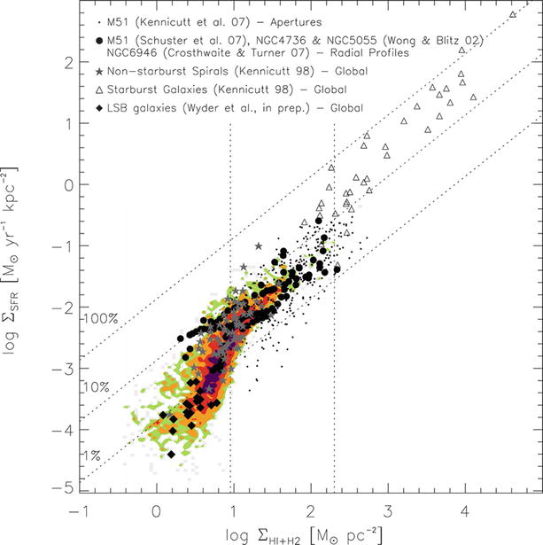
Fig. 3.20

The star formation surface density Σ _SFR as a function of the surface mass density $\varSigma _{\mathrm{HI+H_{2} }}$ of the sum of atomic and molecular gas. The colored-shading shows results from subregions of nearby spiral and late-type dwarf galaxies. Symbols show measurements from either regions or radial bins (dots and black circles), or disk-averaged estimates of normal spiral galaxies (asterisks). Open triangles correspond to starburst galaxies, diamonds to low-surface brightness galaxies. The diagonal lines indicate a star-formation rate in which 1, 10 or 100% of the gas is consumed in star formation within 10⁸ yr. The two vertical lines indicate characteristic values of the projected gas density. Source: F. Bigiel et al. 2008, The Star Formation Law in Nearby Galaxies on Sub-Kpc Scales, AJ 136, 2846, p. 2869, Fig. 15. ©AAS. Reproduced with permission

Due to the apparent absence of star formation in the outer part of spiral galaxies, one often complements this relation with a cut-off at a specific value for Σ _gas.

In Fig. 3.20, recent results of the star-formation rate in galaxies are compiled, ranging from low-surface brightness galaxies (diamonds) to starburst galaxies (open triangles). Here, the gas surface density is taken to be the sum of atomic and molecular gas, where the density of molecular hydrogen is estimated from the abundance of the CO molecule, assuming a constant conversion factor between these two species. The three diagonal lines indicate the star-formation rate at which the available gas reservoir would be consumed in star formation on a time-scale of 10⁸, 10⁹, and 10¹⁰ yr (from top to bottom). A global power-law fit to these data would yield a result very similar to (3.15), with an index N ∼ 1. 4. However, the figure suggests that there are different regimes of star formation activity, indicated by the two vertical lines. The regime shown on the right part of the figure is occupied by starburst galaxies. Using only those, a linear relation between Σ _SFR and Σ _gas seems to describe the data quite well. The regime between the two vertical lines is occupied by normal spiral galaxies, and again, restricting a power-law fit solely to them, a linear relation with N ∼ 1 provides a good approximation. For low values of the gas density (the left part of the figure), the star-formation rate seems to decrease rapidly. Thus, an index N ≈ 1. 4 in the Schmidt–Kennicutt law is obtained as a global fit which makes no distinction between the three different regimes just outlined.

Furthermore, the figure indicates a density threshold in the Schmidt–Kennicutt law. Whereas UV-observations with the GALEX satellite, as well as measurements of Hα emission (which stems from the Hii regions around hot stars), showed that star formation can occur well beyond the optical break radius (see Fig. 3.21), it appears that the corresponding level of star formation is rather low, as indicated also in Fig. 3.20.

A better understanding of the origin of the Schmidt–Kennicutt relation is obtained if one considers the dependence of the star-formation rate on the density of atomic and molecular gas separately. This yields the result that Σ _SFR is essentially proportional to $\varSigma _{\mathrm{H_{2}}}$ . This relation is not very surprising, since we know that star formation occurs in molecular clouds and thus one expects that the molecular gas density controls the star-formation rate.

On the other hand, the star-formation rate exhibits a rather steep dependence on the density of atomic gas, which seems to saturate at a value of about 10 M _⊙ pc⁻², indicated by the left of the vertical lines in Fig. 3.20. But the densities of atomic and molecular gas are not unrelated; molecules form from atoms, and so the dependence of Σ _SFR on the density of atomic gas could be a secondary effect—Σ _SFR depends mostly (or even solely) on the molecular density. The Schmidt–Kennicutt relation can then be understood as a combination of the proportionality between Σ _SFR and $\varSigma _{\mathrm{H_{2}}}$ and the molecular fraction of the gas, which increases with the gas density.

The fact that the starburst galaxies seem to have a higher star-formation rate at a given molecular density may indicate that different physical processes are operating for them; indeed, we have seen before that at least a large fraction of ULIRGs are recent mergers, which are thought to be triggering the starburst.

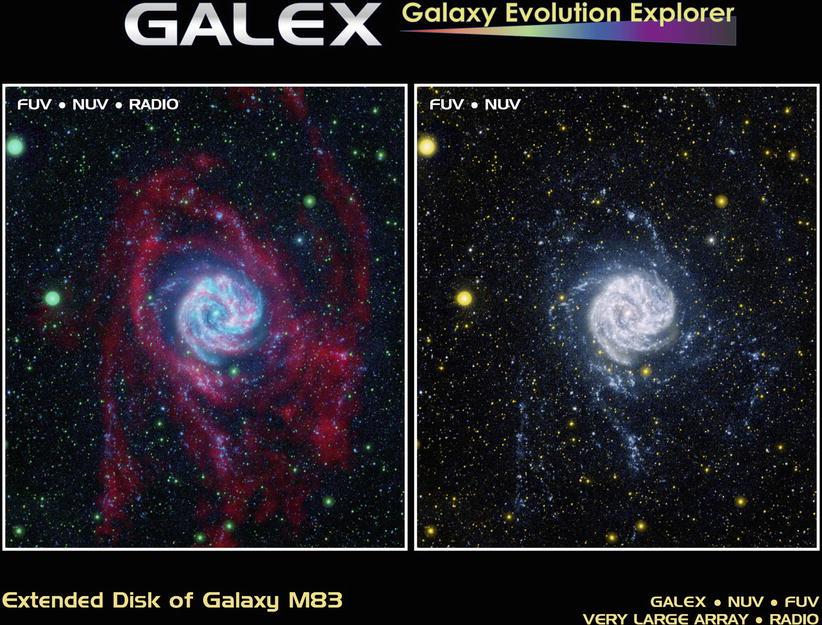
/epubstore/S/P-Schneider/Extragalactic-Astronomy-And-Cosmology/OEBPS/A129044_2_En_3_Fig21_HTML.jpg

Fig. 3.21

The galaxy M83 (the Pinwheel galaxy) seen by the GALEX satellite in UV-light (right), and combined with the 21 cm emission from atomic hydrogen shown in red (left). The gas disk is far more extended than the stellar disk of this face-on spiral galaxy. However, the UV-image clearly shows that new stars are formed even at ∼ 20 kpc from the center of this galaxy, i.e., outside the optical break radius. Credit: NASA/JPL-Caltech/VLA/MPIA

The efficiency of star formation as a function of the surface mass density of gas provides a possible explanation of the observed break in the optical surface brightness of spiral galaxies. However, the fact that the warps observed in neutral hydrogen typically start to occur at this break radius may also imply that the origin of the break may be due to other effects. For example, the disk inside the break radius may have been assembled rather quickly in the formation history of spirals, whereas the matter lying further out could have been added later on in the evolution, e.g., due to the accretion of mass from the surrounding medium.

3.3.4 Rotation curves and dark matter

The rotation curves of other spiral galaxies are easier to measure than that of the Milky Way because we are able to observe them ‘from outside’. These measurements are achieved by utilizing the Doppler effect, where the inclination of the disk, i.e., its orientation with respect to the line-of-sight, has to be accounted for. The inclination angle is determined from the observed axis ratio of the disk, assuming that disks are intrinsically axially symmetric (except for the spiral arms). Mainly the stars and Hi gas in the galaxies are used as luminous tracers, where the observable Hi disk is in general significantly more extended than the stellar disk. Therefore, the rotation curves measured from the 21 cm line typically extend to much larger radii than those from optical stellar spectroscopy.

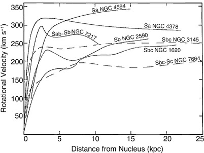
/epubstore/S/P-Schneider/Extragalactic-Astronomy-And-Cosmology/OEBPS/A129044_2_En_3_Fig22_HTML.jpg

Fig. 3.22

Examples of rotation curves of spiral galaxies. They are all flat in the outer region and do not behave as expected from Kepler’s law if the galaxy consisted only of luminous matter. Also striking is the fact that the amplitude of the rotation curve is higher for early-type than for late-type spirals. Source: V. Rubin et al. 1978, Extended rotation curves of high-luminosity spiral galaxies. IV—Systematic dynamical properties, SA through SC, ApJ 225, L107, p. L109, Fig. 3. ©AAS. Reproduced with permission

Like our Milky Way, other spirals also rotate considerably faster in their outer regions than one would expect from Kepler’s law and the distribution of visible matter (see Fig. 3.22).

The rotation curves of spirals do not decrease for R ≥ h _R , as one would expect from the light distribution, but are basically flat. We therefore conclude that spirals are surrounded by a halo of dark matter. The density distribution of this dark halo can be derived from the rotation curves.

To see how the density distribution of the dark matter can be derived from the rotation curves, we employ the force balance between gravitation and centrifugal acceleration, as described by the Kepler rotation law,

$\displaystyle{v^{2}(R) = \mathit{GM}(R)/R\;,}$

from which one directly obtains the mass M(R) within a radius R. The rotation curve expected from the visible matter distribution is⁵

$\displaystyle{v_{\mathrm{lum}}^{2}(R) = \mathit{GM}_{\mathrm{ lum}}(R)/R\;.}$

M _lum(R) can be determined by assuming a plausible value for the mass-to-light ratio M∕L of the luminous matter. This value is obtained either from the spectral light distribution of the stars, together with knowledge of the properties of stellar populations, or by fitting the innermost part of the rotation curve (where the mass contribution of dark matter can presumably be neglected), assuming that M∕L is independent of radius for the stellar population. From this estimate of the mass-to-light ratio, the discrepancy between v _lum ² and v ² yields the distribution of the dark matter, $v_{\mathrm{dark}}^{2} = v^{2} - v_{\mathrm{lum}}^{2} = GM_{\mathrm{dark}}/R$ , or

$\displaystyle{ \fbox{$M_{\mathrm{dark}}(R) = \frac{R} {G}\left [v^{2}(R) - v_{\mathrm{ lum}}^{2}(R)\right ]$}\;. }$

(3.17)

An example of this decomposition of the mass contributions is shown in Fig. 3.23.

/epubstore/S/P-Schneider/Extragalactic-Astronomy-And-Cosmology/OEBPS/A129044_2_En_3_Fig23_HTML.jpg

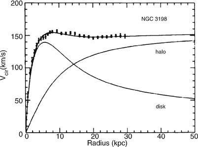
Fig. 3.23

The flat rotation curves of spiral galaxies cannot be explained by visible matter alone. The example of NGC 3198 demonstrates the rotation curve which would be expected from the visible matter alone (curve labeled ‘disk’). To explain the observed rotation curve, a dark matter component has to be present (curve labeled ‘halo’). However, the decomposition into disk and halo mass is not unambiguous because for it to be so it would be necessary to know the mass-to-light ratio of the disk. In the case considered here, a ‘maximum disk’ was assumed, i.e., it was assumed that the innermost part of the rotation curve is produced solely by the visible matter in the disk. Source: T.S. van Albada et al. 1985, Distribution of dark matter in the spiral galaxy NGC 3198, ApJ 295, 305, p. 309, Fig. 4. ©AAS. Reproduced with permission

The decomposition of the rotation curve into a contribution due to the baryonic matter—i.e., mainly stars—and one due to dark matter is not unique, since it depends on the mass-to-light ratio of the stellar population. Assuming M∕L to be constant, one can obtain an upper bound on M∕L by fitting the innermost part of the rotation curve by the stellar contribution only. This then yields the ‘maximum disk’ model for rotation curves. The corresponding values obtained for M∕L are often larger than those obtained from stellar population models, and thus the maximum disk model is not necessary well justified.

The assumption of an almost constant M∕L can be tested in a different way. From stellar dynamics, one can derive a relation between the surface density of the disk, Σ(R), the scale-height of the disk, h _z , and the velocity dispersion of stars perpendicular to the disk, σ _z (R), which in the case of flat rotation curves reads

$\displaystyle{\sigma _{z}(R) = \sqrt{c'\pi G\varSigma (R)h_{z } (R)}\;,}$

where c′ is a constant depending on the vertical profile of the disk; for an exponential profile, $$c' = 3/2$$

. We noted before that the scale-height h _z is observed in edge-on spirals to be independent of R. If M∕L is a constant, independent of R, then the observed brightness profile of disks implies that $\varSigma (R) \propto \exp (-R/h_{R})$ . The foregoing relation then shows that also the velocity dispersion σ _z should follow an exponential in R, but $\propto \exp (-R/2h_{R})$ , due to the square root. Thus, the scale-length on which the velocity dispersion decreases should be twice the scale-length of the surface brightness. Indeed, spectroscopic studies of face-on spirals have shown this to be the case—a result which is consistent with an (almost) constant M∕L of the disk.

The corresponding density profiles of the dark matter halos seem to be flat in the inner region, and decreasing as R ⁻² at large radii. It is remarkable that $\rho \propto R^{-2}$ implies a mass profile M ∝ R, i.e., the mass of the halo increases linearly with the radius for large R. As long as the extent of the halo is undetermined the total mass of a galaxy will be unknown. Since the observed rotation curves are flat out to the largest radius for which 21 cm emission can still be observed, a lower limit for the radius of the dark halo can be obtained, $R_{\mathrm{halo}} \gtrsim 30h^{-1}\mathrm{kpc}$ . Inside the optical radius of a disk, the dark matter comprises about 2/3 of the total mass.

To derive the density profile out to even larger radii, other observable objects in an orbit around the galaxies are needed. Potential candidates for such luminous tracers are satellite galaxies—companions of other spirals, like the Magellanic Clouds are for the Milky Way. Because we cannot presume that these satellite galaxies move on circular orbits around their parent galaxy, conclusions can be drawn based only on a statistical sample of satellites. These analyses of the relative velocities of satellite galaxies around spirals still give no indication of an ‘edge’ to the halo, leading to a lower limit for the radius of $R_{\mathrm{halo}} \gtrsim 100h^{-1}\mathrm{kpc}$ .

Correlations of rotation curves with galaxy properties. The form and amplitude of the rotation curves of spirals are correlated with their luminosity and their Hubble type. The larger the luminosity of a spiral, the steeper the rise of v(R) in the central region, and the larger the maximum rotation velocity v _max. This latter fact indicates that the mass of a galaxy increases with luminosity, as expected. For the characteristic values of the various Hubble types, one finds $v_{\mathrm{max}} \sim 300\,\mathrm{km/s}$ for Sa’s, $v_{\mathrm{max}} \sim 175\,\mathrm{km/s}$ for Sc’s, whereas Irr’s have a much lower v _max ∼ 70 km∕s. For equal luminosity, v _max is higher for earlier types of spirals. However, the shape (not the amplitude) of the rotation curves of different Hubble types is similar, despite the fact that they have a different brightness profile as seen, for instance, from the varying bulge-to-disk ratio. This point is another indicator that the rotation curves cannot be explained by visible matter alone.

Dark matter in ellipticals. For elliptical galaxies the mass estimate, and thus the detection of a possible dark matter component, is significantly more complicated, since the orbits of stars are substantially more complex than in spirals. In particular, the mass estimate from measuring the stellar velocity dispersion via line widths depends on the anisotropy of the stellar orbits, which is a priori unknown. Nevertheless, in recent years it has been unambiguously proven that dark matter also exists in ellipticals. First, the degeneracy between the anisotropy of the orbits and the mass determination was broken by detailed kinematic analysis. Second, in some ellipticals hot gas was detected from its X-ray emission. As we will see in Sect. 6.4 in the context of clusters of galaxies, the temperature of the gas allows an estimate of the depth of the potential well, and therefore the mass. Both methods reveal that ellipticals are also surrounded by a dark halo.

The gravitational lens effect offers another way to determine the masses of galaxies up to very large radii. With this method we cannot study individual galaxies but only the mean mass properties of a galaxy population. The results of these measurements confirm the large size of dark halos in spirals and in ellipticals (see Sect. 7.7).

The quest for dark matter. These results leave us with a number of obvious questions. What is the nature of the dark matter? What are the density profiles of dark halos, how are they determined, and where is the ‘boundary’ of a halo? Does the fact that galaxies with $v_{\mathrm{rot}} \lesssim 100\,\mathrm{km/s}$ have no prominent spiral structure mean that a minimum dark matter mass (or mass concentration) needs to be exceeded in order for spiral arms to form?

Some of these questions will be examined later, but here we point out that the major fraction of the mass of (spiral) galaxies consists of non-luminous matter. The fact that we do not know what this matter consists of leaves us with the question of whether this invisible matter is a new, yet unknown, form of matter. Or is the dark matter less exotic, normal (baryonic) matter that is just not luminous for some reason (for example, because it did not form any stars)? We will see in Chap. 4 that the issue of dark matter is not limited to galaxies, but is also clearly present on a cosmological scale; furthermore, the dark matter cannot be baryonic. A currently unknown form of matter is, therefore, revealing itself in the rotation curves of spirals. We will pick up this issue in Sect. 4.4.6 after we have excluded the possibility that the dark matter is composed of unseen baryons.

3.3.5 Stellar populations and gas fraction

The color of spiral galaxies depends on their Hubble type, with later types being bluer; e.g., one finds B − V ∼ 0. 75 for Sa’s, 0.64 for Sb’s, 0.52 for Sc’s, and 0.4 for Irr’s. This means that the fraction of massive young stars increases along the Hubble sequence towards later spiral types. This conclusion is also in agreement with the findings for the light distribution along spiral arms where we clearly observe active star formation regions in the bright knots in the spiral arms of Sc’s. Furthermore, this color sequence is also in agreement with the decreasing bulge fraction towards later types.

The formation of stars requires gas, and the mass fraction of gas is larger for later types, as can be measured, for instance, from the 21 cm emission of Hi, from Hα and from CO emission. Characteristic values for the ratio $\left \langle M_{\mathrm{gas}}/M_{\mathrm{baryons}}\right \rangle$ are about 0.04 for Sa’s, 0.08 for Sb’s, 0.16 for Sc’s, and 0.25 for Irr’s. It thus appears that early-type spirals have been more efficient in the past in turning their gas into stars. In addition, the fraction of molecular gas relative to the total gas mass is smaller for later Hubble types. The dust mass is less than 1 % of the gas mass, or about 0.1 % of the total baryonic mass.

Dust, in combination with hot stars, is the main source of far-infrared (FIR) emission from galaxies. Sc galaxies emit a larger fraction of FIR radiation than Sa’s, and barred spirals have stronger FIR emission than normal spirals. The FIR emission arises from dust heated by the UV radiation of hot stars and then re-radiating this energy in the form of thermal emission.

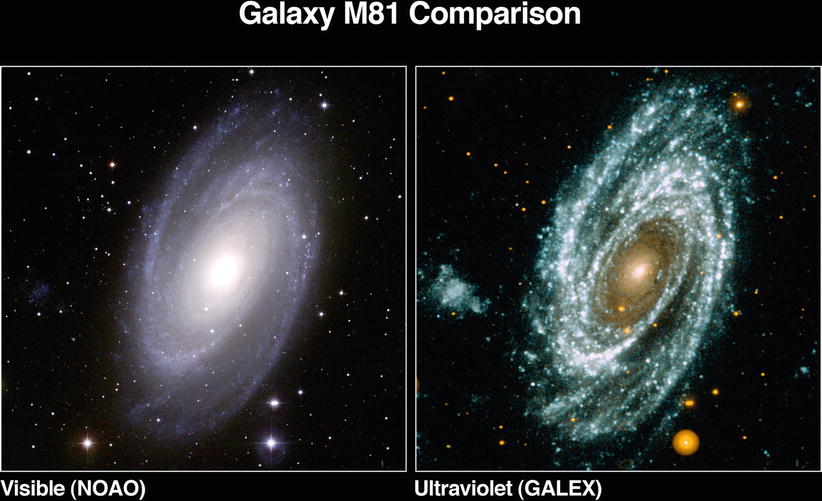
/epubstore/S/P-Schneider/Extragalactic-Astronomy-And-Cosmology/OEBPS/A129044_2_En_3_Fig24_HTML.jpg

Fig. 3.24

The galaxy M81 in optical light (left) and the UV (right). The spiral arms are much more prominent in the UV than in optical light, showing that star formation occurs almost exclusively in spiral arms. Note the absence of any visible UV-emission in the center of the galaxy, indicating the lack of hot stars there. Credit: NASA/JPL-Caltech/NOAO

Dust extinction affects the total optical luminosity that is emitted from a spiral galaxy. Depending on the spatial distribution of the dust relative to that of the stars, the extinction can be direction-dependent. Or in other words: the optical luminosity of a spiral galaxy is not necessarily emitted isotropically, but the mean extinction can be higher if a galaxy is seen edge-on. The occurrence of this effect and its strength can be studied, due to the fact that extinction is related to reddening. By studying the mean color of spirals of fixed near-IR luminosity as a function of observed axis ratio, i.e., as a function of inclination angle, one finds that edge-on spirals are redder than face-on galaxies. From the dependence of the reddening on the inclination angle of a large sample of SDSS galaxies, one finds that the typical extinction of an edge-on spiral is 0.7, 0.6, 0.5 and 0.4 magnitudes in the u-, g-, r-, and i-bands, respectively. Hence, spiral galaxies are not really transparent. This effect seems to be weaker for lower-mass spirals, indicating that their relative dust content is smaller than that of high-mass spirals. This is in accord with the fact that the metallicity of lower-mass galaxies is smaller than that of more massive ones (see Fig. 3.40 below).

A prominent color gradient is observed in spirals: they are red in the center and bluer in the outer regions. We can identify at least two reasons for this trend. The first is a metallicity effect, as the metallicity is increasing inwards and metal-rich stars are redder than metal-poor ones, due to their higher opacity. Second, the color gradient can be explained by star formation. Since the gas fraction in the bulge is lower than in the disk, less star formation takes place in the bulge, resulting in a stellar population that is older and redder in general. Furthermore, it is found that the metallicity of spirals increases with luminosity.

Abundance of globular clusters. The number of globular clusters is higher in early types and in more luminous galaxies. The specific abundance of globular clusters in a galaxy is defined as their number, normalized to a galaxy of absolute magnitude $M_{V } = -15$ . This can be done by scaling the observed number N _t of globular clusters in a galaxy of visual luminosity L _V or absolute magnitude M _V , respectively, to that of a fiducial galaxy with $M_{V } = -15$ , corresponding to a luminosity of L _V = L ₁₅:

$\displaystyle{ S_{N} = N_{\mathrm{t}}\,\frac{L_{15}} {L_{V }} = N_{\mathrm{t}}\,10^{0.4(M_{V }+15)}\;. }$

(3.18)

If the number of globular clusters were proportional to the luminosity (and thus roughly to the stellar mass) of a galaxy, then this would imply a constant S _N . However, this is not the case: For Sa’s and Sb’s we find S _N ∼ 1. 2, whereas S _N ∼ 0. 5 for Sc’s. S _N is larger for ellipticals and largest for cD galaxies.

3.3.6 Spiral structure

The spiral arms are the bluest regions in spirals and they contain young stars and Hii regions. For this reason, the brightness contrast of spiral arms increases as the wavelength of the (optical) observation decreases. In particular, the spiral structure is very prominent in a blue filter, as is shown impressively in Fig. 3.24.

Naturally, the question arises as to the nature of the spiral arms. Probably the most obvious answer would be that they are material structures of stars and gas, rotating around the galaxy’s center together with the rest of the disk. However, this scenario cannot explain spiral arm structure since, owing to the differential rotation, they would wind up much more tightly than observed within only a few rotation periods.

Rather, it is suspected that spiral arms are a wave structure, the velocity of which does not coincide with the physical velocity of the stars. Spiral arms are quasi-stationary density waves, regions of higher density (possibly 10–20 % higher than the local disk environment). If the gas, on its orbit around the center of the galaxy, enters a region of higher density, it is compressed, and this compression of molecular clouds results in an enhanced star formation rate. This accounts for the blue color of spiral arms. Since low-mass (thus red) stars live longer, the brightness contrast of spiral arms is lower in red light, whereas massive blue stars are born in the spiral arms and soon after explode there as SNe. Indeed, only few blue stars are found outside spiral arms.

/epubstore/S/P-Schneider/Extragalactic-Astronomy-And-Cosmology/OEBPS/A129044_2_En_3_Fig25_HTML.jpg

Fig. 3.25

A multi-color view of the spiral galaxy M51, also called the Whirlpool Galaxy, together with its smaller companion NGC 5195 at the top. The image has a size of $2.\!\!^{{\prime}}2 \times 3.\!\!^{{\prime}}2$ and different colors indicate: purple: X-ray emission as observed by Chandra; green: HST optical imaging; red: infrared emission as seen by Spitzer; blue: UV-radiation observed by GALEX. The spiral arms are the location of young stars, and the dusted heated by them is clearly seen from the IR emission. The X-ray emission mainly comes from compact sources like accreting neutron stars and black holes (called X-ray binaries), but also from diffuse emission by hot gas between the young stars. Simulations indicate that the small companion may have passed through M51 in the recent past; in any case, its physical closeness certainly perturbs the gravitational field of M51 which may be the origin for the very pronounced spiral structure and, at the same time, the increased level of star-formation activity, through added compression of the gas. Credit: X-ray: NASA/CXC/Wesleyan Univ./R.Kilgard et al; UV: NASA/JPL-Caltech; Optical: NASA/ESA/S. Beckwith & Hubble Heritage Team (STScI/AURA); IR: NASA/JPL-Caltech/ Univ. of AZ/R. Kennicutt

The generation of spiral arms may be induced by a non-axially symmetric perturbation of the gravitational potential of a disk galaxy. Such perturbation can be due to a massive bar in its center, or by companion galaxies. Figure 3.25 shows a particularly impressive case for the latter possibility, together with a multi-color view of this galaxy. The fact that about 65 % of luminous spirals in the local Universe have a central bar may indicate that bars play an important role in the formation of spiral structure.

In order to better understand density waves we may consider, for example, the waves on the surface of a lake. Peaks at different times consist of different water particles, and the velocity of the waves is by no means the bulk velocity of the water.

3.3.7 Halo gas in spirals

In Sect. 2.3.7 we showed that the disk of the Milky Way is surrounded by gas in its halo, seen as high-velocity clouds in form of neutral hydrogen, absorption by highly ionized species, and X-ray emission from a hot gas. These properties are not unique to the Galaxy.

Corona in spirals. Hot gas resulting from supernovae and their subsequent evolution may expand out of the disk and thereby be ejected to form a hot gaseous halo of a spiral galaxy. We might therefore suspect that such a ‘coronal’ gas exists outside the galactic disk. While the existence of this coronal gas has long been suspected, the detection of its X-ray emission was first made possible with the ROSAT satellite in the early 1990s. However, the limited angular resolution of ROSAT rendered the distinction between diffuse emission and clusters of discrete sources difficult. Finally, the Chandra observatory unambiguously detected the coronal gas in a number of spiral galaxies. As an example, Fig. 3.26 shows the spiral galaxy NGC 4631.

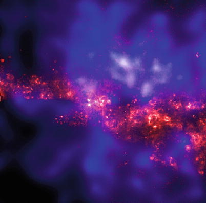
/epubstore/S/P-Schneider/Extragalactic-Astronomy-And-Cosmology/OEBPS/A129044_2_En_3_Fig26_HTML.jpg

Fig. 3.26

The spiral galaxy NGC 4631. The optical (HST) image of the galaxy is shown in red; the many luminous areas are regions of very active star formation. The SN explosions of massive stars eject hot gas into the halo of the galaxy. This gas (at a temperature of T ∼ 10⁶ K) emits X-ray radiation, shown as the blue diffuse emission as observed by the Chandra satellite. The image has a size of 2. ^′ 5. Credit: X-ray: NASA/UMass/D. Wang et al., Optical: NASA/HST/D. Wang et al.; Research article: D. Wang et al. 2001, Chandra Detection of a Hot Gaseous Corona around the Edge-on Galaxy NGC 4631, ApJ 555, L99

Neutral hydrogen, in the form of high-velocity clouds, has been detected outside the disk of many spiral galaxies, generally within ∼ 10 kpc of the disk. It is estimated that about 25 % of luminous spirals have more than 10⁸ M _⊙ of neutral hydrogen gas outside the disk. In those cases where the Hi mass is large it can be related to tidal features or streams indicating the accretion of smaller galaxies—like the Magellanic stream in our Milky Way, which contains most of the neutral hydrogen in our halo.

Ionized gas. Detecting ionized gas and hot gas outside the plane of spiral galaxies is in fact easier in external galaxies than it is in the Milky Way. Whereas emission of Hα is detected outside of the disk is other spirals, the clearest signals are due to absorption lines in the spectra of background sources, usually quasars, which can trace gas with low column density. When the redshifts of the absorption lines are correlated with the position of foreground galaxies, one can study the extend and covering factor of the gas giving rise to this absorption. One finds that the Lyα absorption has a covering factor of almost unity within ∼ 300 kpc of luminous galaxies, and the covering factor of Mgii absorption within 100 kpc is about 50 %. Hence, warm ionized gas extends to large separation from galaxies. In addition, in star-forming galaxies, one also finds highly ionized species (like Ovi) at large distance from the disk.

Taken together, we find that the halo gas in other spirals shares the properties of that in the Milky Way. The gaseous halo is a busy place, where one meets metal-enriched gas driven out by energetic processes in the galactic disk, and low-metallicity gas falling in from larger distances, providing new raw material for continued star formation. The various phases of the gas in halos are essentially in pressure equilibrium, i.e., their density scales inversely to their temperature.

3.4 Scaling relations

The properties of a galaxy are characterized by a number of quantities, such as luminosity, size, mass, rotational velocity or velocity dispersion, color, star-formation rate etc. At first sight one might think that galaxies can exist where these different quantities take on a large range of values. However, this is not the case: The properties of isolated galaxies seem to be determined by just a few parameters, from which the others follow.

As a first example of that fact, we will show in this section that the kinematic properties of spirals and ellipticals are closely related to their luminosity. As we shall discuss below, spirals follow the Tully–Fisher relation (Sect. 3.4.1), whereas elliptical galaxies obey the Faber–Jackson relation (Sect. 3.4.2) and are located in the fundamental plane (Sect. 3.4.3). These scaling relations are a very important tool for distance estimations, as will be discussed in Sect. 3.9. Furthermore, these scaling relations express relations between galaxy properties which any successful model of galaxy evolution must be able to explain. Here we will describe these scaling relations and discuss their physical origin.

3.4.1 The Tully–Fisher relation

Using 21 cm observations of spiral galaxies, in 1977 R. Brent Tully and J. Richard Fisher found that the maximum rotation velocity of spirals is closely related to their luminosity, following the relation

$\displaystyle{ \fbox{$L \propto v_{\mathrm{max}}^{\alpha }$}\;, }$

(3.19)

where the power-law index (i.e., the slope) of the Tully–Fisher relation is about α ∼ 4. The larger the wavelength of the filter in which the luminosity is measured, the smaller the dispersion of the Tully–Fisher relation (see Fig. 3.27). This is to be expected because radiation at larger wavelengths is less affected by dust absorption and by the current star formation rate, which may vary to some extent between individual spirals. Furthermore, it is found that the value of α increases with the wavelength of the filter: The Tully–Fisher relation is steeper in the red, which follows from the fact that more massive, or more luminous galaxies—i.e., those with larger v _max—are redder, as can be seen from Fig. 3.7. The dispersion of galaxies around the relation (3.19) in the near-infrared (e.g., in the H-band) is about 10 %.

/epubstore/S/P-Schneider/Extragalactic-Astronomy-And-Cosmology/OEBPS/A129044_2_En_3_Fig27_HTML.jpg

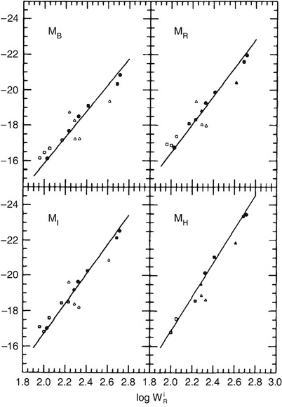
Fig. 3.27

The Tully–Fisher relation for galaxies in the Local Group (dots), in the Sculptor group (triangles), and in the M81 group (squares). The absolute magnitude is plotted as a function of the width of the 21 cm profile which indicates the maximum rotation velocity (see Fig. 3.28). Filled symbols represent galaxies for which independent distance estimates were obtained, either from RR Lyrae stars, Cepheids, or planetary nebulae. For galaxies represented by open symbols, the average distance of the respective group is used. The solid line is a fit to similar data for the Ursa-Major cluster, together with data of those galaxies for which individual distance estimates are available (filled symbols). The larger dispersion around the mean relation for the Sculptor group galaxies is due to the group’s extent along the line-of-sight. Source: M.J. Pierce & R.B. Tully 1992, Luminosity-line width relations and the extragalactic distance scale. I—Absolute calibration, ApJ 387, 47, p. 51, Fig. 1. ©AAS. Reproduced with permission

Because of this close correlation, the luminosity of spirals can be estimated quite precisely by measuring the rotational velocity. The determination of the (maximum) rotational velocity is independent of the galaxy’s distance. By comparing the luminosity, as determined from the Tully–Fisher relation, with the measured flux, one can then estimate the distance of the galaxy —without utilizing the Hubble relation!

The measurement of v _max is obtained either from a spatially resolved rotation curve, by measuring v _rot(θ), which can be done with optical spectroscopy or, for relatively nearby galaxies, also with spatially resolved 21 cm spectroscopy. Alternatively, one can observe an integrated spectrum of the 21 cm line of Hi that has a Doppler width corresponding to about 2v _max (see Fig. 3.28). The Tully–Fisher relation shown in Fig. 3.27 was determined by measuring the width of the 21 cm line.

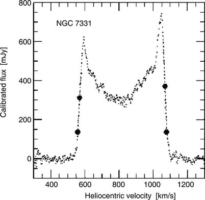
/epubstore/S/P-Schneider/Extragalactic-Astronomy-And-Cosmology/OEBPS/A129044_2_En_3_Fig28_HTML.jpg

Fig. 3.28

21 cm profile of the galaxy NGC 7331. The bold dots indicate 20 and 50 % of the maximum flux; these are of relevance for the determination of the line width from which the rotational velocity is derived. Source: L.M. Macri et al. 2000, A Database of Tully–Fisher Calibrator Galaxies, ApJS 128, 461, p. 467, Fig. 5. ©AAS. Reproduced with permission

Explaining the Tully–Fisher-relation. The shapes of the rotation curves of spirals are very similar to each other, in particular with regard to their flat behavior in the outer part. The flat rotation curve implies

$\displaystyle{ \fbox{$M = \frac{v_{\mathrm{max}}^{2}R} {G} $}\;, }$

(3.20)

where the value of the distance R from the center of the galaxy is chosen to be in the range of the flat part of the rotation curve, i.e., where $v_{\mathrm{rot}}(R) \approx V _{\mathrm{max}}$ . We note that the exact value of R is not important; of course, M = M(R) in (3.20). By re-writing (3.20),

$\displaystyle{ L = \left (\frac{M} {L} \right )^{-1}\,\frac{v_{\mathrm{max}}^{2}R} {G} \;, }$

(3.21)

and replacing R by the mean surface brightness $\left \langle I\right \rangle = L/R^{2}$ , we obtain

$\displaystyle{ L = \left (\frac{M} {L} \right )^{-2}\left ( \frac{1} {G^{2}\,\left \langle I\right \rangle }\right )\,v_{\mathrm{max}}^{4}\;. }$

(3.22)

This is the Tully–Fisher relation if M∕L and $\left \langle I\right \rangle$ are the same for all spirals. As discussed previously, the latter is in fact suggested by Freeman’s law (Sect. 3.3.2). Since the shapes of rotation curves for spirals seem to be very similar, the radial dependence of the ratio of luminous to dark matter may also be quite similar among spirals. Furthermore, since the mass-to-light ratios of a stellar population as measured from the red or infrared emission do not depend strongly on its age, the constancy of M∕L could also be valid if dark matter is included.

Although the line of argument presented above is far from a rigorous derivation of the Tully–Fisher-relation, it nevertheless makes the existence of such a scaling relation plausible.

Mass-to-light ratio of spirals. We are unable to determine the total mass of a spiral because the extent of the dark halo is unknown. Thus we can measure M∕L only within a fixed radius. We shall define this radius as R ₂₅, the radius at which the surface brightness attains the value of 25 mag/arcsec² in the B-band⁶; then spirals follow the relation

$\displaystyle{ \fbox{$\log \left (\frac{R_{25}} {\mathrm{kpc}}\right ) = -0.249M_{B} - 4.00$}\;, }$

(3.23)

independently of their Hubble type. Within R ₂₅ one finds $M/L_{B} = 6.2$ for Sa’s, 4.5 for Sb’s, and 2.6 for Sc’s. This trend does not come as a surprise because late types of spirals contain more young, blue and luminous stars.

The baryonic Tully–Fisher relation. The above ‘derivation’ of the Tully–Fisher relation is based on the assumption of a constant M∕L value, where M is the total mass (i.e., including dark matter). Let us assume that (1) the ratio of baryons to dark matter is constant, and furthermore that (2) the stellar populations in spirals are similar, so that the ratio of stellar mass to luminosity is a constant. Even under these assumptions we would expect the Tully–Fisher relation to be valid only if the gas does not, or only marginally, contribute to the baryonic mass. However, low-mass spirals contain a significant fraction of gas, so we should expect that the Tully–Fisher relation does not apply to these galaxies. Indeed, it is found that spirals with a small $v_{\mathrm{max}} \lesssim 100\,\mathrm{km/s}$ deviate significantly from the Tully–Fisher relation—see Fig. 3.29a.

/epubstore/S/P-Schneider/Extragalactic-Astronomy-And-Cosmology/OEBPS/A129044_2_En_3_Fig29_HTML.jpg

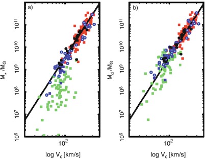
Fig. 3.29

(a) The mass contained in stars as a function of the rotational velocity V _c for spirals. This stellar mass is computed from the luminosity by multiplying it with a suitable stellar mass-to-light ratio which depends on the chosen filter and which can be calculated from stellar population models. This is the ‘classical’ Tully–Fisher relation. Squares and circles denote galaxies for which V _c was determined from the 21 cm line width or from a spatially resolved rotation curve, respectively. The colors of the symbols indicate the filter band in which the luminosity was measured: H (red), K’ (black), I (green), B (blue). (b) Instead of the stellar mass, here the sum of the stellar and gaseous mass is plotted. The gas mass was derived from the flux in the 21 cm line, $M_{\mathrm{gas}} = 1.4M_{\mathrm{HI}}$ , corrected for helium and metals. The line in both plots is the Tully–Fisher relation with a slope of α = 4. Source: S. McGaugh et al. 2000, The Baryonic Tully-Fisher Relation, ApJ 533, L99, p. L100, Fig. 1. ©AAS. Reproduced with permission

Since the luminosity is approximately proportional to the stellar mass, L ∝ M _∗, the Tully–Fisher relation is a relation between v _max and M _∗. Adding the mass of the gas, which can be determined from the strength of the 21 cm line and molecular emission, to the stellar mass, a much tighter correlation is obtained, see Fig. 3.29b. It reads

$\displaystyle{ \fbox{$M_{\mathrm{disk}} = 2 \times 10^{9}\,h^{-2}\,M_{ \odot }\left ( \frac{v_{\mathrm{max}}} {100\,\mathrm{km/s}}\right )^{4}$}\;, }$

(3.24)

and is valid over five orders of magnitude in disk mass $M_{\mathrm{disk}} = M_{{\ast}} + M_{\mathrm{gas}}$ . If no further baryons exist in spirals (such as, e.g., MACHOs), this close relation means that the ratio of baryons and dark matter in spirals is constant over a very wide mass range.

3.4.2 The Faber–Jackson relation

A relation for elliptical galaxies, analogous to the Tully–Fisher relation, was found by Sandra Faber and Roger Jackson. They discovered that the velocity dispersion in the center of ellipticals, σ ₀, scales with luminosity (see Fig. 3.30),

$\displaystyle{ \fbox{$L \propto \sigma _{0}^{4}$}\;,\;\;\mathrm{or}\;\;\fbox{$\log (\sigma _{ 0}) = -0.1M_{B} +\mathrm{ const.}$}\;. }$

(3.25)

‘Deriving’ the Faber–Jackson scaling relation is possible under the same assumptions as for the Tully–Fisher relation. However, the dispersion of ellipticals about this relation is larger than that of spirals about the Tully–Fisher relation.

/epubstore/S/P-Schneider/Extragalactic-Astronomy-And-Cosmology/OEBPS/A129044_2_En_3_Fig30_HTML.jpg

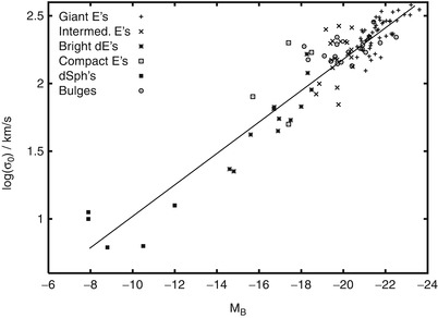
Fig. 3.30

The Faber–Jackson relation expresses a relation between the velocity dispersion and the luminosity of elliptical galaxies. It can be derived from the virial theorem. Data from R. Bender et al. 1992, ApJ 399, 462

3.4.3 The fundamental plane

The Tully–Fisher and Faber–Jackson relations specify a connection between the luminosity and a kinematic property of galaxies. As we discussed previously, various relations exist between the parameters of elliptical galaxies. Thus one might wonder whether a relation exists between observables of elliptical galaxies for which the dispersion is smaller than that of the Faber–Jackson relation. Such a relation was indeed found and is known as the fundamental plane.

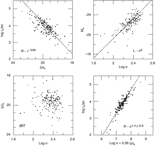
/epubstore/S/P-Schneider/Extragalactic-Astronomy-And-Cosmology/OEBPS/A129044_2_En_3_Fig31_HTML.jpg

Fig. 3.31

Projections of the fundamental plane onto different two-parameter planes. Upper left: the relation between radius and mean surface brightness within the effective radius. Upper right: Faber–Jackson relation. Lower left: the relation between mean surface brightness and velocity dispersion shows the fundamental plane viewed from above. Lower right: the fundamental plane viewed from the side—the linear relation between radius and a combination of surface brightness and velocity dispersion. Source: J. Kormendy & S. Djorgovski 1989, Surface photometry and the structure of elliptical galaxies, ARA&A 27, 235, Fig. 2, p. 255. Reprinted, with permission, from the Annual Review of Astronomy & Astrophysics, Volume 27 ©1989 by Annual Reviews www.annualreviews.org

To explain this relation, we will consider the various relations between the parameters of ellipticals. In Sect. 3.2.2 we saw that the effective radius of normal ellipticals and cD’s, i.e., excluding dwarfs, is related to the luminosity (see Fig. 3.10). This implies a relation between the surface brightness and the effective radius,

$\displaystyle{ \fbox{$R_{\mathrm{e}} \propto \left \langle I\right \rangle _{\mathrm{e}}^{-0.83}$}\;, }$

(3.26)

where $\left \langle I\right \rangle _{\mathrm{e}}$ is the average surface brightness within the effective radius, so that

$\displaystyle{ \fbox{$L = 2\pi R_{\mathrm{e}}^{2}\left \langle I\right \rangle _{\mathrm{ e}}$}\;. }$

(3.27)

From this, a relation between the luminosity and $\left \langle I\right \rangle _{\mathrm{e}}$ results,

$\displaystyle\begin{array}{rcl} L& \propto & R_{\mathrm{e}}^{2}\left \langle I\right \rangle _{\mathrm{ e}} \propto \left \langle I\right \rangle _{\mathrm{e}}^{-0.66}\;\mbox{ or approximately} \fbox{$\left \langle I\right \rangle _{\mathrm{ e}} \propto L^{-1.5}$}\,.{}\end{array}$

(3.28)

Hence, more luminous ellipticals have smaller surface brightnesses, as is also shown in Fig. 3.10. By means of the Faber–Jackson relation, L is related to σ ₀, the central velocity dispersion, and therefore, σ ₀, $\left \langle I\right \rangle _{\mathrm{e}}$ , and R _e are related to each other. The distribution of elliptical galaxies in the three-dimensional parameter space $(R_{\mathrm{e}},\left \langle I\right \rangle _{\mathrm{e}},\sigma _{0})$ is located close to a plane defined by

$\displaystyle{ \fbox{$R_{\mathrm{e}} \propto \sigma _{0}^{1.4}\left \langle I\right \rangle _{\mathrm{ e}}^{-0.85}$}\;. }$

(3.29)

Writing this relation in logarithmic form, we obtain

$\displaystyle{ \fbox{$\log R_{\mathrm{e}} = 0.34\left \langle \mu \right \rangle _{\mathrm{e}} + 1.4\log \sigma _{0} +\mathrm{ const.}$}\;, }$

(3.30)

where $\left \langle \mu \right \rangle _{\mathrm{e}}$ is the average surface brightness within R _e, measured in mag/arcsec². Equation (3.30) defines a plane in this three-dimensional parameter space that is known as the fundamental plane (FP). Different projections of the fundamental plane are displayed in Fig. 3.31.

How can this be explained? The mass within R _e can be derived from the virial theorem, $M \propto \sigma _{0}^{2}R_{\mathrm{e}}$ . Combining this with (3.27) yields

$\displaystyle{ R_{\mathrm{e}} \propto \frac{L} {M}\,\frac{\sigma _{0}^{2}} {\left \langle I\right \rangle _{\mathrm{e}}}\;. }$

(3.31)

If the mass-to-light ratio M∕L was the same for all ellipticals, then (3.31) deviates significantly from the observed fundamental plane (3.29). This deviation is often called the tilt of the fundamental plane. This tilt can be accounted for if the mass-to-light ratio varies systematically with the galaxy mass. To wit, (3.31) agrees with the FP in the form of (3.29) if

$\displaystyle{ \frac{L} {M}\,\frac{\sigma _{0}^{2}} {\left \langle I\right \rangle _{\mathrm{e}}} \propto \frac{\sigma _{0}^{1.4}} {\left \langle I\right \rangle _{\mathrm{e}}^{0.85}}\;,}$

$\displaystyle{\frac{M} {L} \propto \frac{\sigma _{0}^{0.6}} {\left \langle I\right \rangle _{\mathrm{e}}^{0.15}} \propto \frac{M^{0.3}} {R_{\mathrm{e}}^{0.3}}\,\frac{R_{\mathrm{e}}^{0.3}} {L^{0.15}} \;.}$

Hence, the FP follows from the virial theorem provided

$\displaystyle{ \left (\frac{M} {L} \right ) \propto M^{0.2}\quad \mathrm{or}\quad \left (\frac{M} {L} \right ) \propto L^{0.25}\;,\quad \mathrm{respectively,} }$

(3.32)

i.e., if the mass-to-light ratio of galaxies increases slightly with mass. Since the luminosity is approximately proportional to the stellar mass, in particular for an old stellar population as found in ellipticals, then (3.32) implies that the ratio of dynamical mass M to stellar mass increases with mass. This increase of M∕L with mass could in principle have its origin in a changing M _∗∕L with increasing mass or luminosity, since we have seen in Fig. 3.7 that more luminous red galaxies are somewhat redder, indicating an older stellar population, which in turn would imply an increasing M _∗∕L. However, this effect is far too small to explain the tilt of the fundamental plane. In addition, the tilt is also seen if the fundamental plane is studied at near-IR wavelengths, for which M _∗∕L is much less age dependent. Hence we conclude that the tilt in the fundamental plane is not related to properties of the stellar population.

Like the Tully–Fisher relation, the fundamental plane is an important tool for distance estimations, as will be discussed more thoroughly later.

3.4.4 D _n -σ relation

Another scaling relation for ellipticals which is of substantial importance in practical applications is the D _n -σ relation. D _n is defined as the mean diameter of an ellipse within which the average surface brightness I _n corresponds to a value of 20.75 mag/arcsec² in the B-band. If we now assume that all ellipticals have a self-similar brightness profile, $I(R) = I_{\mathrm{e}}\,f(R/R_{\mathrm{e}})$ , with f(1) = 1, then the luminosity within D _n can be written as

$\displaystyle\begin{array}{rcl} I_{n}\left (\frac{D_{n}} {2} \right )^{2}\pi & =& 2\pi I_{\mathrm{ e}}\int _{0}^{D_{n}/2}\mathrm{d}R\;R\,f(R/R_{\mathrm{ e}}) {}\\ & =& 2\pi I_{\mathrm{e}}R_{\mathrm{e}}^{2}\int _{ 0}^{D_{n}/(2R_{\mathrm{e}})}\mathrm{d}x\,x\,f(x)\;, {}\\ \end{array}$

where in the last step we changed the integration variable to $x = R/R_{\mathrm{e}}$ . For a de Vaucouleurs profile we have approximately f(x) ∝ x ^−1. 2 in the relevant range of radius. Computing the integral with this expression, we obtain

$\displaystyle{ D_{n} \propto R_{\mathrm{e}}\,I_{\mathrm{e}}^{0.8}\;. }$

(3.33)

Replacing R _e by the fundamental plane (3.29) then results in

$\displaystyle{D_{n} \propto \sigma _{0}^{1.4}\,\left \langle I\right \rangle _{\mathrm{ e}}^{-0.85}\,I_{\mathrm{ e}}^{0.8}\;.}$

Since we assumed a self-similar brightness profile, we have $\left \langle I\right \rangle _{\mathrm{e}} \propto I_{\mathrm{e}}$ , and thus we finally find

$\displaystyle{ \fbox{$D_{n} \propto \sigma _{0}^{1.4}\,I_{\mathrm{ e}}^{0.05}$}\;. }$

(3.34)

This implies that D _n is nearly independent of I _e and only depends on σ ₀. The D _n -σ relation (3.34) describes the properties of ellipticals considerably better than the Faber–Jackson relation and, in contrast to the fundamental plane, it is a relation between only two observables. Empirically, we find that ellipticals follow the normalized D _n -σ relation

$\displaystyle{ \frac{D_{n}} {\mathrm{kpc}} = 2.05\left ( \frac{\sigma _{0}} {100\,\mathrm{km/s}}\right )^{1.33}\;, }$

(3.35)

and they scatter around this relation with a relative width of about 15 %.

3.4.5 Summary: Properties of galaxies on the Hubble sequence

After having discussed the basic properties of the two main types of galaxies and some of the scaling relations they obey, this is a good place to pause and summarize the main points:

Most luminous galaxies in the local Universe fit onto the Hubble sequence; they are either ellipticals, spirals, or belong to the class of S0 galaxies, which shares some properties with the two other classes.
Ellipticals and spirals differ not only in their morphology, but in several other respects, for example: (1) Spirals contain a sizable fraction of gas, whereas the gas-to-stellar mass ratio in ellipticals is much smaller. As a consequence, (2) spirals have ongoing star formation, ellipticals not, or only very little. As a further consequence, (3) the light of elliptical galaxies is substantially redder than that of spirals. Obviously, the morphology of galaxies and the properties of their stellar populations are strongly correlated.
The stars in spirals have a very ordered motion, moving around the galactic center on nearly circular orbits in a common orbital plane, having a velocity dispersion that is much smaller than the orbital velocity; the stars in the disk are called ‘dynamically cold’. In contrast, the motion of stars in ellipticals is largely random, with fairly little coherent velocity; they are dynamically hot.
Some elliptical galaxies show clear signs of complex structure, which are interpreted as indications of past interaction with other galaxies. In contrast, the disks of spirals are very thin, which means that they have been largely unperturbed for a long while in the past.
The rotation curves of spiral galaxies are almost flat for large radii, in contrast to what would be expected from the visible mass distribution that declines exponentially outwards. This implies that there is more matter than seen in stars and gas—the galaxies are embedded in a halo of dark matter. Whereas for elliptical galaxies the radial density distribution is more difficult to probe, the presence of dark matter has been verified also for ellipticals.
Both, spirals and ellipticals, follow scaling relations which connect their luminous properties (luminosity or surface brightness) with their dynamical properties (rotational velocity or velocity dispersion). Hence, the formation and evolution of galaxies and their stellar populations must proceed in a way as to place them onto these scaling relations.

Next, we will consider the properties of stellar populations in somewhat more detail, since they are a key in relating the observed luminous properties of galaxies to their underlying baryonic component.

3.5 Population synthesis

The light of normal galaxies originates from stars. Stellar evolution is largely understood, and the spectral radiation of stars can be calculated from the theory of stellar atmospheres. If the distribution of the number density of stars is known as a function of their mass, chemical composition, and evolutionary stage, we can compute the light emitted by them. The theory of population synthesis aims at interpreting the spectrum of galaxies as a superposition of stellar spectra. We have to take into account the fact that the distribution of stars changes over time; e.g., massive stars leave the main sequence after several 10⁶ yr, the number of luminous blue stars thus decreases, which means that the spectral distribution of the population also changes in time. The spectral energy distribution of a galaxy thus reflects its history of star formation and stellar evolution. For this reason, simulating different star formation histories and comparing them with observed galaxy spectra provides important clues for understanding the evolution of galaxies. In this section, we will discuss some aspects of the theory of population synthesis; this subject is of tremendous importance for our understanding of galaxy spectra.

3.5.1 Model assumptions

The processes of star formation are not understood in detail; for instance, it is currently impossible to compute the mass spectrum of a group of stars that jointly formed in a molecular cloud. Obviously, high-mass and low-mass stars are born together and form young (open) star clusters. The mass spectra of these stars are determined empirically from observations.

The initial mass function (IMF) is defined as the initial mass distribution at the time of birth of the stars, such that ϕ(m) dm specifies the fraction of stars in the mass interval of width dm around m, where the distribution is normalized,

$\displaystyle{\fbox{$\int _{m_{\mathrm{L}}}^{m_{\mathrm{U}} }\mathrm{d}m\;m\,\phi (m) = 1M_{\odot }$}\;.}$

The integration limits are not well defined. Typically, one uses m _L ∼ 0. 1M _⊙ because stars less massive than ≈ 0. 08M _⊙ do not ignite their hydrogen (and are thus brown dwarfs), and $m_{\mathrm{U}} \sim 100M_{\odot }$ , because considerably more massive stars are not observed. Whereas such very massive stars would in any case be difficult to observe because of their very short lifetime, the theory of stellar structure tells us that more massive stars can probably not form a stable configuration due to excessive radiation pressure. The shape of the IMF is also subject to uncertainties; in most cases, the Salpeter-IMF is used,

$\displaystyle{ \fbox{$\phi (m) \propto m^{-2.35}$}\;, }$

(3.36)

as obtained from investigating the stellar mass spectrum in young star clusters. It is by no means clear whether a universal IMF exists, or whether it depends on specific conditions like metallicity, the mass of the galaxy, cosmic epoch, or other parameters. Given the difficulties of determining the shape of the IMF, apparent variations of the IMF with epoch or environment may be attributed to other effect, such as the specifics of the star-formation history in galaxies. Therefore, there seems to be no clear direct indication that the IMF varies with environment. However, as will be discussed in Chap. 10, some properties of high-redshift galaxies are very difficult to understand if their IMF would be the same as in our neighborhood. It has therefore been suggested that the IMF in starbursts is different from that of quiescent star formation such as we are experiencing in the Milky Way.

Fig. 3.32

(a) Evolutionary tracks in the HRD for stars of different masses, as indicated by the numbers near the tracks (in units of M _⊙). The ZAMS (zero age main sequence) is the place of birth in the HRD; evolution moves stars away from the main sequence. Depending on the mass, they explode as a core-collapse SN (for M ≥ 8M _⊙) or end as a white dwarf (WD). Prior to this, they move along the red giant branch (RGB) and the asymptotic giant branch (AGB). (b) Isochrones at different times, indicated in units of 10⁹ yr. An isochrone (for a given time t) is a curve connecting the location of stars in the HRD which all have the same age t. Thus, an isochrone shows the distribution of stars from a single star-formation event after a time t. The upper main sequence is quickly depopulated by the rapid evolution of massive stars, whereas the red giant branch is populated over time. Source: S. Charlot 1996, Spectral Evolution of Galaxies, Lecture Notes in Physics 470, Springer-Verlag, p. 53

The Salpeter-IMF seems to be a good description for stars with M ≳ 1M _⊙, whereas the IMF for less massive stars is flatter. Note that, due to the steep slope of the IMF, most of the stellar mass is contained in low-mass stars. However, since the luminosity of main-sequence stars depends strongly on mass, approximately as L ∝ M ³, most of the luminosity comes from high-mass stars (see Problem 3.2).

The star-formation rate is the gas mass that is converted into stars per unit time,

$\displaystyle{\psi (t) = -\frac{\mathrm{d}M_{\mathrm{gas}}} {\mathrm{d}t} \;.}$

The metallicity Z of the ISM defines the metallicity of the newborn stars, and the stellar properties in turn depend on Z. During stellar evolution, metal-enriched matter is ejected into the ISM by stellar winds, planetary nebulae, and SNe, so that Z(t) is an increasing function of time. This chemical enrichment must be taken into account in population synthesis studies in a self-consistent form.

Let S _λ, Z (t′) be the emitted energy per wavelength and time interval, normalized to an initial total mass of 1M _⊙, emitted by a group of stars of initial metallicity Z and age t′. The function $S_{\lambda,Z(t-t')}(t')$ , which describes this emission at any point t in time, accounts for the different evolutionary tracks of the stars in the Hertzsprung–Russell diagram (HRD)—see Appendix B.2. It also accounts for their initial metallicity (i.e., at time t − t′), where the latter follows from the chemical evolution of the ISM of the corresponding galaxy. Then the total spectral luminosity of this galaxy at a time t is given by

$\displaystyle{ F_{\lambda }(t) =\int _{ 0}^{t}\mathrm{d}t'\;\psi (t - t')\,S_{\lambda,Z(t-t')}(t')\;, }$

(3.37)

thus by the convolution of the star formation rate with the spectral energy distribution of the stellar population. In particular, F _λ (t) depends on the star formation history.

3.5.2 Evolutionary tracks in the HRD; integrated spectrum

In order to compute S _{λ, Z(t−t′)}(t′), models for stellar evolution and stellar atmospheres are needed. As a reminder, Fig. 3.32a displays the evolutionary tracks in the HRD. Each track shows the position of a star with specified mass in the HRD and is parametrized by the time since its formation. Positions of equal time in the HRD are called isochrones and are shown in Fig. 3.32b. As time proceeds, fewer and fewer massive stars exist because they quickly leave the main sequence and end up as supernovae or white dwarfs. The number density of stars along the isochrones depends on the IMF. The spectrum $S_{\lambda,Z(t-t')}(t')$ is then the sum over all spectra of the stars on an isochrone—see Fig. 3.33b.

Fig. 3.33

(a) Comparison of the spectrum of a main sequence star with a black body spectrum of equal effective temperature. The opacity of the stellar atmosphere causes clear deviations from the Planck spectrum in the UV/optical. (b) Spectrum of a stellar population with Solar metallicity that was instantaneously born a time t ago; t is given in units of 10⁹ yr. Source: S. Charlot 1996, Spectral Evolution of Galaxies, Lecture Notes in Physics 470, Springer-Verlag, p. 53

In the beginning, the spectrum and luminosity of a stellar population are dominated by the most massive stars, which emit intense UV radiation. But after ∼ 10⁷ yr, the flux below 1000 Å is diminished significantly, and after ∼ 10⁸ yr, it hardly exists any more. At the same time, the flux in the NIR increases because the massive stars evolve into red supergiants.

For $10^{8}\,\mathrm{yr} \lesssim t \lesssim 10^{9}\,\mathrm{yr}$ , the emission in the NIR remains high, whereas short-wavelength radiation is more and more diminished. After ∼ 10⁹ yr, red giant stars (RGB stars) account for most of the NIR production. After ∼ 3 × 10⁹ yr, the UV radiation increases again slightly, due to blue stars on the horizontal branch into which stars evolve after the AGB phase, and due to white dwarfs which are hot when they are born. Between an age of 4 and 13 billion years, the spectrum of a stellar population evolves fairly little.

Of particular importance is the spectral break located at about 4000 Å which becomes visible in the spectrum after a few 10⁷ yr. This break is caused by a strongly changing opacity of stellar atmospheres at this wavelength, mainly due to strong transitions of singly ionized calcium and the Balmer lines of hydrogen. This 4000 Å-break is one of the most important spectral properties of the continuum stellar emission in galaxies; as we will discuss in Sect. 9.1.2, it allows us to estimate the redshifts of early-type galaxies from their photometric properties—so-called photometric redshift estimates.

3.5.3 Color evolution

Detailed spectra of galaxies are often not available. Instead we have photometric images in different broadband filters, since the observing time required for spectroscopy is substantially larger than for photometry. In addition, modern wide-field cameras can obtain photometric data of numerous galaxies simultaneously. From the theory of population synthesis we can derive photometric magnitudes by multiplying model spectra with the filter functions, i.e., the transmission curves of the color filters used in observations, and then integrating over wavelength (A.25). Hence the spectral evolution implies a color evolution, as is illustrated in Fig. 3.34a.

Fig. 3.34

(a) For the same stellar population as in Fig. 3.33b, the upper two graphs show the colors B − V and V − K as a function of age. The lower two graphs show the mass-to-light ratio M∕L in two color bands in Solar units. The solid curves show the total M∕L (i.e., including the mass that is later returned into the ISM), whereas the dashed curves show the M∕L of the stars itself. (b) The fraction of B- (top) and K-luminosity (bottom) contributed by stars in their different phases of stellar evolution (MS: main sequence; CHeB: core helium burning stars; SGB: sub-giant branch). Source: S. Charlot 1996, Spectral Evolution of Galaxies, Lecture Notes in Physics 470, Springer-Verlag, p. 53

For a young stellar population the color evolution is rapid and the population becomes redder, again because the hot blue stars have a higher mass and thus evolve quickly in the HRD. For the same reason, the evolution is faster in B − V than in V − K. It should be mentioned that this color evolution is also observed in star clusters of different ages. The mass-to-light ratio M∕L also increases with time because M remains constant while L decreases.

As shown in Fig. 3.34b, the blue light of a stellar population is always dominated by main sequence stars, although at later stages a noticeable contribution also comes from horizontal branch stars. The NIR radiation is first dominated by stars burning helium in their center (this class includes the supergiant phase of massive stars), later by AGB stars, and after ∼ 10⁹ yr by red giants. Main sequence stars never contribute more than 20 % of the light in the K-band. The fact that M∕L _K varies only little with time implies that the NIR luminosity is a good indicator for the total stellar mass: the NIR mass-to-light ratio is much less dependent on the age of the stellar population than that for bluer filters.

3.5.4 Star formation history and galaxy colors

Up to now, we have considered the evolution of a stellar population of a common age (called an instantaneous burst of star formation). However, star formation in a galaxy takes place over a finite period of time. We expect that the star formation rate decreases over time because more and more matter is bound in stars and thus no longer available to form new stars. Since the star formation history of a galaxy is a priori unknown, it needs to be parametrized in a suitable manner. A ‘standard model’ of an exponentially decreasing star formation rate was established for this,

$\displaystyle{ \fbox{$\psi (t) =\tau ^{-1}\,\exp \left [-(t - t_{\mathrm{ f}})/\tau \right ]\,\mathrm{H}(t - t_{\mathrm{f}})$}\;, }$

(3.38)

where τ is the characteristic duration and t _f the onset of star formation. The last factor in (3.38) is the Heaviside step function, H(x) = 1 for x ≥ 0, H(x) = 0 for x < 0. This Heaviside step function accounts for the fact that ψ(t) = 0 for t < t _f. We may hope that this simple model describes the basic aspects of a stellar population. Results of this model are plotted in Fig. 3.35a in a color-color diagram.

From the diagram we find that the colors of the population depend strongly on τ. Specifically, galaxies do not become very red if τ is large because their star formation rate, and thus the fraction of massive blue stars, does not decrease sufficiently. The colors of Sb spirals, for example, are not compatible with a constant star formation rate—except if the total light of spirals is strongly reddened by dust absorption (but there are good reasons why this is not the case). To explain the colors of early-type galaxies we need $\tau \lesssim 4 \times 10^{9}\,\mathrm{yr}$ . In general, one deduces from these models that a substantial evolution to redder colors occurs for $t \gtrsim \tau$ . Since the luminosity of a stellar population in the blue spectral range decreases quickly with the age of the population, whereas increasing age affects the red luminosity much less, we conclude:

The spectral distribution of galaxies is mainly determined by the ratio of the star formation rate today to the mean star formation rate in the past, $\psi (\mathrm{today})/\left \langle \psi \right \rangle$ .

One of the achievements of this standard model is that it explains the colors of present day galaxies, which have an age ≳ 10 billion years. However, this model is not unambiguous because other star formation histories ψ(t) can be constructed with which the colors of galaxies can be modeled as well.

3.5.5 Metallicity, dust, and Hii regions

Predictions of the model depend on the metallicity Z—see Fig. 3.35b. A small value of Z results in a bluer color and a smaller M∕L ratio in the V band. The age and metallicity of a stellar population are degenerate in the sense that an increase in the age by a factor X is nearly equivalent to an increase of the metallicity by a factor 0. 65X with respect to the color of a population. The age estimate of a population from observed colors therefore strongly depends on the assumed value for Z. However, this degeneracy may be broken by taking several colors, or information from absorption-line spectroscopy, into account.

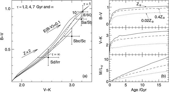
/epubstore/S/P-Schneider/Extragalactic-Astronomy-And-Cosmology/OEBPS/A129044_2_En_3_Fig35_HTML.jpg

Fig. 3.35

(a) Evolution of colors between $0 \leq t \leq 17 \times 10^{9}\,\mathrm{yr}$ for a stellar population with star-formation rate given by (3.38), for five different values of the characteristic time scale τ (τ = ∞ is the limiting case for a constant star formation rate)—see solid curves. The typical colors for four different morphological types of galaxies are plotted. For each τ, the evolution begins at the lower left, i.e., as a blue population in both color indices. In the case of constant star formation, the population never becomes redder than Irr’s; to achieve redder colors, τ has to be smaller. The dashed line connects points of t = 10¹⁰ yr on the different curves. Here, a Salpeter IMF and Solar metallicity was assumed. The shift in color obtained by doubling the metallicity is indicated by an arrow, as well as that due to an extinction coefficient of $$E(B - V ) = 0.1$$

; both effects will make galaxies appear redder. (b) The dependence of colors and M∕L on the metallicity of the population. Source: S. Charlot 1996, Spectral Evolution of Galaxies, Lecture Notes in Physics 470, Springer-Verlag, p. 53

Intrinsic dust absorption will also change the colors of a population. This effect cannot be easily accounted for in the models because it depends not only on the properties of the dust but also on the geometric distribution of dust and stars. For example, it makes a difference whether the dust in a galaxy is homogeneously distributed or concentrated in a thin disk. Empirically, it is found that galaxies show strong extinction during their active phase of star formation, whereas normal galaxies are less affected by extinction, with early-type galaxies (E/S0) affected the least.

From the optical luminosity and colors of a stellar population, one can estimate its stellar mass. Obviously, the stellar mass is the product of the mass-to-light ratio and the luminosity, and M∕L can be estimated from the broad-band color—see Fig. 3.34. The presence of dust of course affects these estimates. However, its two effects conspire in a particular way: dust reduces the luminosity that escapes from a stellar population, and reddens the optical light. The latter effect thus leads to the larger estimate of the mass-to-light ratio. As a reasonable approximation, the reduction of the luminosity and the increase of the M∕L-estimate compensate such that the estimated stellar mass is fairly insensitive to the presence of dust.

Besides stellar light, the emission by Hii regions also contributes to the light of galaxies. It is found, though, that after ∼ 10⁷ yr the emission from gas nebulae only marginally contributes to the broad-band colors of galaxies. However, this nebular radiation is the origin of emission lines in the spectra of galaxies. Therefore, emission lines are used as diagnostics for the star formation rate and the metallicity in a stellar population.

Whereas one might expect that stellar evolution is well understood, as well as the theory of stellar atmospheres where the radiation emitted from stars is formed, the models of population synthesis are still in a state of development. Fairly recently, it was found that a specific type of star—the thermally pulsating AGB stars (TP-AGB)—can significantly affect the emission of a stellar population with ages between 0.5 and 2 Gyr. Depending on how the contribution from these stars are treated in population synthesis models, the resulting predicted spectral flux, and integrated galaxy luminosity, of single-age stellar populations in the above age range can differ substantially. The effect is much smaller in stellar populations with a slowly varying formation rate; therefore, the uncertainties mainly concern post-starburst stellar populations. Hence, if a galaxy is observed about 1 Gyr after a starburst, the estimated amount of star formation during this burst depends on how the population synthesis model treats the effects of TP-AGB stars.

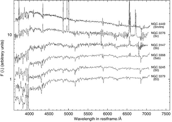
/epubstore/S/P-Schneider/Extragalactic-Astronomy-And-Cosmology/OEBPS/A129044_2_En_3_Fig36_HTML.jpg

Fig. 3.36

Spectra of galaxies of different types, where the spectral flux is plotted logarithmically in arbitrary units. The spectra are ordered according to the Hubble sequence, with early types at the bottom and late-type spectra at the top. Data from R. Kennicutt 1992, ApJS 79, 255

3.5.6 The spectra of galaxies

At the end of this section we shall consider the typical spectra of different galaxy types. They are displayed for six galaxies of different Hubble types in Fig. 3.36. To make it easier to compare them, they are all plotted in a single diagram where the logarithmic flux scale is arbitrarily normalized (since this normalization does not affect the shape of the spectra).

It is easy to recognize the general trends in these spectra: the later the Hubble type, (1) the bluer the overall spectral distribution, (2) the stronger the emission lines, (3) the weaker the absorption lines, and (4) the smaller the 4000 Å-break in the spectra. From the above discussion, we would also expect these trends if the Hubble sequence is considered an ordering of galaxy types according to the characteristic age of their stellar population or according to their star-formation rate. Elliptical and S0 galaxies essentially have no star formation activity, which renders their spectral energy distribution dominated by red stars. Furthermore, in these galaxies there are no Hii regions where emission lines could be generated. The old stellar population produces a pronounced 4000 Å break, which corresponds to a jump by a factor of ∼ 2 in the spectra of early-type galaxies. It should be noted that the spectra of ellipticals and S0 galaxies are quite similar.

By contrast, Sc spirals and irregular galaxies have a spectrum which is dominated by emission lines, where the Balmer lines of hydrogen as well as nitrogen and oxygen lines are most pronounced. The relative strength of these emission lines are characteristic for Hii-regions, implying that most of this line emission is produced in the ionized regions surrounding young stars. For irregular galaxies, the spectrum is nearly totally dominated by the stellar continuum light of hot stars and the emission lines from Hii-regions, whereas clear contributions by cooler stars can be identified in the spectra of Sc spiral galaxies.

The spectra of Sa and Sb galaxies form a kind of transition between those of early-type galaxies and Sc galaxies. Their spectra can be described as a superposition of an old stellar population generating a red continuum with absorption features and a young population with its blue continuum and its emission lines. This can be seen in connection with the decreasing contribution of the bulge to the galaxy luminosity towards later spiral types.

The properties of the spectral light distribution of different galaxy types, as briefly discussed here, is described and interpreted in the framework of population synthesis. This gives us a detailed understanding of stellar populations as a function of the galaxy type. Extending these studies to spectra of high-redshift galaxies allows us to draw conclusions about the evolutionary history of their stellar populations.

3.5.7 Summary

After this somewhat lengthy section, we shall summarize the most important results of population synthesis here:

A simple model of star formation history reproduces the colors of today’s galaxies fairly well.
(Most of) the stars in elliptical and S0 galaxies are old—the earlier the Hubble type, the older the stellar population.
Detailed models of population synthesis provide information about the star formation history, and predictions by the models can be compared with observations of galaxies at high redshift (and thus smaller age).

We will frequently refer to results from population synthesis in the following chapters. For example, we will use them to interpret the colors of galaxies at high redshifts and the different spatial distributions of early-type and late-type galaxies (see Chap. 6). Also, we will present a method of estimating the redshift of galaxies from their broad-band colors (photometric redshifts). As a special case of this method, we will discuss the efficient selection of galaxies at very high redshift (Lyman-break galaxies, LBGs, see Chap. 9). Because the color and luminosity of a galaxy are changing even when no star formation is taking place, tracing back such a passive evolution allows us to distinguish this passive aging process from episodes of star formation and other processes.

3.6 The population of luminous galaxies

We started this chapter with the classification of galaxies, according to morphology and according to their colors. After discussing the properties of elliptical and spiral galaxies in some detail, we are now ready to ask the obvious question: what is the relation between ellipticals and spirals on the one hand, and red and blue galaxies on the other? How are these two classification schemes related? Furthermore, we may look for other global properties of galaxies that either correlate strongly with color, or with morphology.

The Sérsic brightness profile. As we have seen, the brightness distribution of disks follows in general an exponential profile, whereas bulges of disk galaxies and the light profile of ellipticals are better described with a de Vaucouleurs profile. Thus, the brightness profiles of galaxies are expected to correlate well with their morphological type. J. Sérsic introduced the brightness profile

$\displaystyle{ \log \left (\frac{I(R)} {I_{\mathrm{e}}} \right ) = -b_{n}\left [\left ( \frac{R} {R_{\mathrm{e}}}\right )^{1/n} - 1\right ]\;, }$

(3.39)

hence called Sérsic brightness profile , where n is called the Sérsic index. As was the case for the de Vaucouleurs profile, the effective radius R _e is chosen such that half of the luminosity comes from within the circle of radius R _e. The coefficient b _n must be chosen such that this property is fulfilled; to good approximation, one finds b _n ≈ 1. 999n − 0. 327. I _e is the surface brightness at R _e. If n = 4, (3.39) reduces to the de Vaucouleurs law, whereas for n = 1, an exponential surface brightness distribution is obtained; in this way, the Sérsic law provides a generalization of, and includes these two brightness profiles. The larger n, the more concentrated the light profile is in the central part, and at the same time, the higher is the surface brightness for large R; see Fig. 3.37.

/epubstore/S/P-Schneider/Extragalactic-Astronomy-And-Cosmology/OEBPS/A129044_2_En_3_Fig37_HTML.jpg

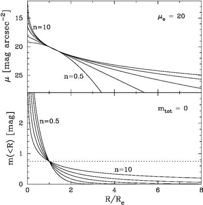
Fig. 3.37

The Sérsic profile, plotted for various values of n. In the upper panel, the surface brightness is plotted as a function of R∕R _e, where all profiles are chosen to have the same brightness at R _e. The straight line (second from bottom) is the exponential profile, n = 1. In the lower panel, the enclosed flux within R is displayed, again normalized such that all profiles agree at R _e, which is equivalent to say that all profiles have the same total magnitude. Source: A.W. Graham & S.P. Driver 2005, A concise reference to (projected) Sersic R ^1∕n quantities, including Concentration, Profile Slopes, Petrosian indices, and Kron Magnitudes, astro-ph/0503176; Credit: NASA/JPL-Caltech

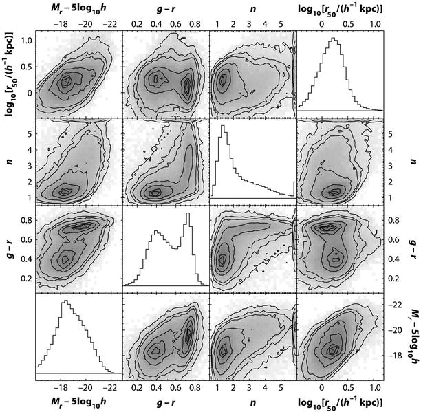
/epubstore/S/P-Schneider/Extragalactic-Astronomy-And-Cosmology/OEBPS/A129044_2_En_3_Fig38_HTML.jpg

Fig. 3.38

The distribution of photometric properties of galaxies, as obtained from the Sloan Digital Sky Survey. The greyscales and contours in the off-diagonal panels show the number of galaxies in each two-dimensional bin; the darker the bins, the higher is the galaxy number. These distributions are shown for six combinations of the four photometric parameters: absolute magnitude in the r-band M _r (note that for a dimensionless Hubble constant of h = 0. 71, 5logh ≈ −0. 74), the color g − r, the Sérsic index n, and the effective radius, here called r ₅₀. Note that panels in the upper left part are just mirror images of those in the lower right part. The panels on the diagonal show the number distribution of galaxies with respect to the four photometric parameters. Source: M.R. Blanton & J. Moustakas, 2009, Physical Properties and Environments of Nearby Galaxies, ARA&A 47, 159, p. 162, Fig. 1. Reprinted, with permission, from the Annual Review of Astronomy & Astrophysics, Volume 47 ©2009 by Annual Reviews www.annualreviews.org

The Sérsic profile provides a convenient parametrization of the brightness profiles of galaxies, and can be used to classify them, by getting the best fit of their light profile with (3.39). In this way, n, R _e and I _e is obtained. The fit is not expected to be a good one in all cases; for example, if one considers an Sa spiral galaxy, for which the bulge contributes substantially to the total light, a single Sérsic profile for both the (de Vaucouleurs) bulge and the (exponential) disk will not necessarily provide an accurate fit. In this case, one would expect that n lies between 1 and 4, depending on the relative strength of the bulge. Indeed, n correlates well with the bulge-to-disk ratio of galaxies. For nearby galaxies, where the brightness profile is well resolved, multi-component Sérsic models are usually fitted, with an inner one for describing the bulge component and the outer one fitting the disk.

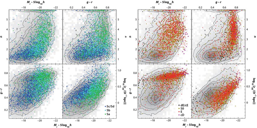
/epubstore/S/P-Schneider/Extragalactic-Astronomy-And-Cosmology/OEBPS/A129044_2_En_3_Fig39_HTML.jpg

Fig. 3.39

Distribution of galaxies that are morphologically classified as spirals (left) and early-type galaxies (right), in the same parameter space as in Fig. 3.38. The greyscale and contours are same as in Fig. 3.38. Different types of galaxies are distinguished by differently colored points. Source: M.R. Blanton & J. Moustakas, 2009, Physical Properties and Environments of Nearby Galaxies, ARA&A 47, 159, p. 174, 186, Fig. 8, 12. Reprinted, with permission, from the Annual Review of Astronomy & Astrophysics, Volume 47 ©2009 by Annual Reviews www.annualreviews.org

Photometric properties of local galaxies. The SDSS provided the first very large survey of galaxies with homogeneous photometry and spectroscopy, in particular redshift information. Therefore, this survey allowed us to study the statistical properties of galaxy properties in great detail. In Fig. 3.38, the distribution of ∼ 77 000 galaxies with z ≤ 0. 05 is shown in terms of photometric parameters, characterizing the luminosity, color, size, and brightness profile of these galaxies. The distribution in absolute magnitude, shown in the lower left panel, indicates that the galaxy sample becomes incomplete for objects less luminous than M _r ∼ −19, owing to the flux limit of the spectroscopic sample in the SDSS.⁷ Lower luminosity galaxies are in the sample only if they are very close to us.

Red sequence, blue cloud, and green valley. The color-magnitude plot (left column, third panel from top) shows essentially the same distribution as in Fig. 3.7, except that here the g − r color is shown (and the absolute magnitude axis is reversed). Galaxies show a clearly bimodal distribution in this space, with two peaks corresponding to luminous red galaxies, and less luminous blue galaxies; these are often called red-sequence galaxies and blue-cloud galaxies, respectively. This bimodality is also seen in the distribution of galaxy colors, shown by the histogram in the second diagonal panel from the bottom left. The spread of red-sequence galaxies in color is much less than that of the blue-cloud galaxies. Thus, the color of red galaxies is very well defined, also seen by the small slope of their distribution in the color-magnitude diagram. The galaxies located between the red sequence and the blue cloud are called green-valley galaxies.

This result is not so surprising after the discussion in Sect. 3.5: the (red) color of an old stellar population depends only little on its exact age. The interpretation of the narrow distribution of the red sequence in color is thus that these galaxies have an old stellar population, with essentially no or very little recent star formation. The slight trend of somewhat redder colors for more luminous galaxies within the red sequence, seen in the color-magnitude diagram, can be due to somewhat higher ages of more luminous galaxies, or higher metallicities. The spread in color of the blue-cloud galaxies presumably reflect different levels of star-formation activities, leading to different mean stellar ages of the population. Here the trend in the color-magnitude diagram is much stronger than for the red sequence: the characteristic color of blue-cloud galaxies correlates significantly with luminosity, in that more luminous galaxies tend to be redder than less luminous ones.

Interestingly, the Sérsic index n correlates clearly with galaxy color, as shown by the second panel in the second row of Fig. 3.38. For blue galaxies, it is strongly concentrated around n ≈ 1, corresponding to an exponential brightness profile. For red galaxies, there is a much broader distribution; in particular, the de Vaucouleurs value n = 4 is not singled out. There is a clear trend that more luminous galaxies are more concentrated than less luminous ones. This behavior holds for the galaxy population as a whole, as well as separately for the blue-cloud and red-sequence galaxies. Consequently, n increases towards redder galaxies on the red sequence. The effective radius correlates strongly with galaxy luminosity, in that more luminous galaxies are more extended.

How does this relate to the Hubble sequence? For a subset of the nearby galaxies in SDSS, a classification by optical morphology is available. These galaxies are plotted in the same photometric parameter space as considered before in Fig. 3.39, where on the left-hand side, spiral galaxies are shown, and early-type galaxies on the right-hand side. The underlying gray-scale and contours are identical with those in Fig. 3.38, showing the distribution of the whole galaxy population.

Considering the color-magnitude diagram (lower left panels) first, we see that the overwhelming majority of early-type galaxies lie on the red sequence, and those that do not are mostly dwarf galaxies. Very few early-type galaxies are located in the blue cloud, which implies that the blue-cloud galaxies are essentially all (star-forming) spirals. This behavior was expected, given our earlier discussion of elliptical galaxies in which ellipticals were described as objects with essentially no ongoing star formation, and consequently red colors.

Surprisingly, the converse is not true: not all red-sequence galaxies are early types. In fact, spiral galaxies are not confined to the blue cloud, but occupy a rather extended region in the color-magnitude diagram, with a clear dependence on type: late-type spirals (Sc/Sd) are on average bluer and less luminous than earlier types. This is expected, based on the relative importance of the (red) bulge compared to the (blue) disk. The influence of relative bulge strength can also be seen in the distribution with respect to Sérsic index n, which clusters around n ∼ 1 for late-type spirals, but has a broad distribution for earlier types. However, the bulge-to-disk ratio is not the only quantity that determines the color and Sérsic index of spirals. As is seen from the distribution of n for early-type galaxies, it is not true that the spheroidal component of galaxies is generally described by a de Vaucouleurs profile with n = 4, but n varies substantially among ellipticals. Furthermore, the color of spirals can be substantially affected by dust in their ISM.

The distribution of galaxies with respect to their effective radius (lower right panels) shows a clear tendency—the earlier the galaxy type, the smaller is the effective radius at fixed absolute magnitude. This behavior is not independent of the relation between galaxy types and Sérsic index, with later types having smaller n. Since n describes the concentration of the light distribution, the light of early-type galaxies (with larger n) is more concentrated than that of later types, implying a smaller effective radius at fixed luminosity.

The color-magnitude distribution of S0 galaxies is almost indistinguishable from that of elliptical galaxies, whereas their concentration index n is clearly smaller than that of E’s. The latter is expected due to their disk component.

Metallicity. Owing to the availability of spectral information for the SDSS galaxies, the distribution of spectral properties of galaxies can be studied. The metallicity of galaxies, as determined from their relative oxygen abundance [O/H], correlates very strongly with stellar mass, in that more massive galaxies contain more metals (see Fig. 3.40). In particular, the dispersion of galaxy metallicity around the mean trend is fairly small. We will see in Sect. 3.7 that this correlation is expected from models of the chemical evolution of galaxies.

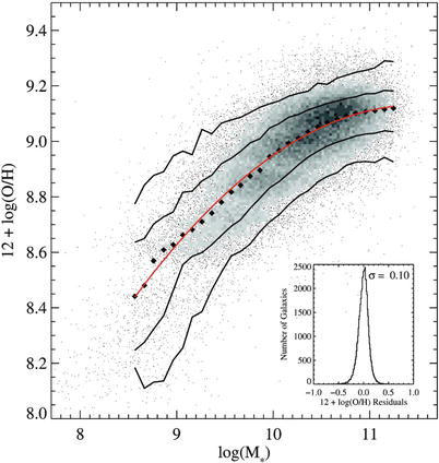
/epubstore/S/P-Schneider/Extragalactic-Astronomy-And-Cosmology/OEBPS/A129044_2_En_3_Fig40_HTML.jpg

Fig. 3.40

For some 53 000 star-forming galaxies in the SDSS, the oxygen abundance of the interstellar medium is plotted against the stellar mass M _∗. The density of points is indicated by the greyscales in high-density regions, and individual galaxies are plotted in the less populated parts of the diagram. The black diamonds represent the median of the distribution of [O/H] in small bins of M _∗, whereas the red curve shows a fit through these data points. The solid black curves enclose 68 and 95 % of the distribution. There is an unambiguous trend of increased metallicity with stellar mass. The small inset shows the distribution of galaxy metallicities around the fit curve; the dispersion of galaxy metallicity around this mean curve is fairly small. Above $M_{{\ast}}\sim 3 \times 10^{10}M_{\odot }$ , the relation between metallicity and stellar mass seems to saturate. Source: C.A. Tremonti et al. 2004, The Origin of the Mass-Metallicity Relation: Insights from 53,000 Star-forming Galaxies in the Sloan Digital Sky Survey, ApJ 613, 898, p. 907, Fig. 6. ©AAS. Reproduced with permission

Most interesting is the bimodal distribution of galaxies with respect to their 4000 Å-break, which is a reliable indicator of the luminosity-weighted mean age of a stellar population (see Sect. 3.5.2). Galaxies with a stellar mass $\gtrsim 1.5 \times 10^{10}h^{-2}M_{\odot }$ typically have a strong 4000 Å-break, whereas lower-mass galaxies have a weak break. The bimodality in this distribution is very similar to that in the color-magnitude diagram, and presumably has the same origin: more massive galaxies have an older stellar population, which renders them redder and having a stronger 4000 Å-break.

Summary. The statistical investigation of a large sample of luminous nearby galaxies yielded remarkable insights into properties of the galaxy population.

The distribution of galaxies is well structured. Instead of filling the possible space of photometric and spectroscopic parameters more or less uniformly, they are confined largely to well-defined sequences. Indeed, it seems that their properties are largely determined by their luminosity or stellar mass: the more massive a galaxy is, the more likely it is that it is red, has a strong 4000 Å-break, a large Sérsic index, high metallicity, and a large effective radius. Conversely, less luminous galaxies are mostly blue, show a weak 4000 Å-break, have n ∼ 1, smaller metallicity and smaller effective radius.

There is a more or less strong dispersion of galaxy properties around these general trends, which is probably caused by differences in the recent star-formation activity and different dust contents; in addition, the color of spiral galaxies depends somewhat on their inclination, as discussed in Sect. 3.3.5. The variation of galaxy properties is considerably larger for spirals, whereas early-type galaxies form a fairly uniform population. The dependence of the galaxy population on environmental effects will be discussed in Sect. 6.7.

3.7 Chemical evolution of galaxies

During its evolution, the chemical composition of a galaxy changes. Thus the observed metallicity yields information about the galaxy’s star formation history. We expect the metallicity Z to increase with star-formation rate, integrated over the lifetime of the galaxy. We will now discuss a simple model of the chemical evolution of a galaxy, which will provide insight into some of the principal aspects.

We assume that at the formation epoch of the stellar population of a galaxy, at time t = 0, no metals were present; hence Z(0) = 0. Furthermore, the galaxy did not contain any stars at the time of its birth, so that all baryonic matter was in the form of gas. In addition, we consider the galaxy as a closed system out of which no matter can escape or be added later on by processes of accretion or merger. Finally, we assume that the time-scales of the stellar evolution processes that lead to the metal enrichment of the galaxy are small compared to the evolutionary time-scale of the galaxy. Under these assumptions, we can now derive a relation between the metallicity and the gas content of a galaxy.

Of the total mass of a newly formed stellar population, part of it is returned to the ISM by supernova explosions and stellar winds. We define this fraction as R, so that the fraction $\alpha = (1 - R)$ of a newly-formed stellar population remains enclosed in stars, i.e., it no longer takes part in the further chemical evolution of the ISM. The value of α depends on the IMF of the stellar population and can be computed from models of population synthesis. Furthermore, let q be the ratio of the mass in metals, which is produced by a stellar population and then returned into the ISM, and the initial total mass of the population. The yield $y = q/\alpha$ is defined as the ratio of the mass in metals that is produced by a stellar population and returned into the ISM, and the mass that stays enclosed in the stellar population. The yield can also be calculated from population synthesis models. If ψ(t) is the star formation rate as a function of time, then the mass of all stars formed in the history of the galaxy is given by

$\displaystyle{S(t) =\int _{ 0}^{t}\mathrm{d}t'\;\psi (t')\;,}$

and the total mass that remains enclosed in stars is s(t) = α S(t). Since we have assumed a closed system for the baryons, the sum of gas mass g(t) and stellar mass s(t) is a constant, namely the baryon mass of the galaxy,

$\displaystyle{ g(t) + s(t) = M_{\mathrm{b}}\;\; \Rightarrow \;\; \frac{\mathrm{d}g} {\mathrm{d}t} + \frac{\mathrm{d}s} {\mathrm{d}t} = 0\;. }$

(3.40)

The mass of the metals in the ISM is gZ; it changes when stars are formed. Through this formation, the mass of the ISM and thus also that of its metals decreases. On the other hand, metals are also returned into the ISM by processes of stellar evolution. Under the above assumption that the time scales of stellar evolution are small, this return occurs virtually instantaneously. The metals returned to the ISM are composed of metals that were already present at the formation of the stellar population—a fraction R of these will be returned—and newly formed metals. Together, the total mass of the metals in the ISM obeys the evolution equation

$\displaystyle{\frac{\mathrm{d}(gZ)} {\mathrm{d}t} =\psi \left (RZ + q\right ) - Z\psi \;,}$

where the last term specifies the rate of the metals extracted from the ISM in the process of star formation and the first term describes the return of metals to the ISM by stellar evolution processes. Since $\mathrm{d}S/\mathrm{d}t =\psi$ , this can also be written as

$\displaystyle{\frac{\mathrm{d}(gZ)} {\mathrm{d}S} = (R - 1)Z + q = q -\alpha Z\;.}$

Dividing this equation by α and using s = α S and the definition of the yield, $y = q/\alpha$ , we obtain

$\displaystyle{ \frac{\mathrm{d}(gZ)} {\mathrm{d}s} = \frac{\mathrm{d}g} {\mathrm{d}s}Z + g\frac{\mathrm{d}Z} {\mathrm{d}s} = y - Z\;. }$

(3.41)

From (3.40) it follows that $\mathrm{d}g/\mathrm{d}s = -1$ and $\mathrm{d}Z/\mathrm{d}s = -\mathrm{d}Z/\mathrm{d}g$ , and so we obtain a simple equation for the metallicity,

$\displaystyle\begin{array}{rcl} g\frac{\mathrm{d}Z} {\mathrm{d}g} & =& \frac{\mathrm{d}Z} {\mathrm{d}\ln g} = -y \\ \Rightarrow \;\; Z(t)& =& -y\,\ln \left (\frac{g(t)} {M_{\mathrm{b}}} \right ) = -y\,\ln (\mu _{\mathrm{g}})\;,{}\end{array}$

(3.42)

where $\mu _{\mathrm{g}} = g/M_{\mathrm{b}}$ is the fraction of baryons in the ISM, and where we chose the integration constant such that at the beginning, when μ _g = 1, the metallicity was Z = 0. From this relation, we can now see that with decreasing gas content in a galaxy, the metallicity will increase; in our simple model this increase depends only on the yield y. Since y can be calculated from population synthesis models with a typical value of y ∼ 10⁻², (3.42) is a well-defined relation.

If (3.42) is compared with observations of galaxies, one finds that they follow the general trend predicted by (3.42). More gas-rich galaxies tend to have smaller metallicities. For example, the metallicities of Sa-galaxies is in general higher than those of later-type spirals which contain a higher gas mass fraction. However, in detail there are strong deviations from (3.42), which are particularly prominent for low-mass galaxies. While the assumption of an instantaneous evolution of the ISM is fairly well justified, we know from structure formation in the Universe (Chap. 7) that galaxies are by no means isolated systems: their mass continuously changes through accretion and merging processes. In addition, the kinetic energy transferred to the ISM by supernova explosions causes an outflow of the ISM, in particular in low-mass galaxies where the gas is not strongly gravitationally bound. These outflows are directly observed in terms of galactic winds from star-forming galaxies, and may explain the deviations from (3.42) by up to a factor of 10 for the low-mass galaxies. An analysis of star-forming galaxies in the SDSS indicates that galaxies with stellar masses below $\sim 4 \times 10^{9}M_{\odot }$ can lose more than half their metals by outflows. Of course, the observed deviations from relation (3.42) allow us to draw conclusions about these accretion and wind processes.

Also, from observations in our Milky Way we find indications that the model of the chemical evolution sketched above is too simplified. This is known as the G-dwarf problem. The model described above predicts that about half of the F- and G-main sequence stars should have a metallicity of less than a quarter of the Solar value. These stars have a long lifetime on the main sequence, so that many of those observed today should have been formed in the early stages of the Galaxy. Thus, in accordance with our model they should have very low metallicity. However, a low metallicity is in fact observed in only very few of these stars. The discrepancy is far too large to be explained by selection effects. Rather, observations show that the chemical evolution of our Galaxy must have been substantially more complicated than described by our simple model. Indeed, we saw in Sect. 2.3.7 that there is clear evidence for infalling gas towards the Galactic plane, providing new and rather low-metallicity material for star formation.

3.8 Black holes in the centers of galaxies

As we have seen in Sect. 2.6.3, the Milky Way harbors a black hole in its center. Furthermore, it is generally accepted that the energy for the activity of AGNs is generated by accretion onto a black hole (see Sect. 5.3). Thus, the question arises as to whether all (or most) galaxies contain a supermassive black hole (SMBH) in their nuclei. We will pursue this question in this section and show that SMBHs are very abundant indeed. This result then instigates further questions: what distinguishes a ‘normal’ galaxy from an AGN if both have a SMBH in the nucleus? Is it the mass of the black hole, the rate at which matter is accreted onto it, or the efficiency of the mechanism which is generating the energy?

We will start with a concise discussion of how to search for SMBHs in galaxies, then present some examples for the discovery of such SMBHs. Finally, we will discuss the very tight relationship between the mass of the SMBH and the properties of the stellar component of a galaxy.

3.8.1 The search for supermassive black holes

What is a black hole? A technical answer is that a black hole is the simplest solution of Einstein’s theory of general relativity which describes the gravitational field of a point mass. Less technically—though sufficient for our needs—we may say that a black hole is a point mass, or a compact mass concentration, with an extent smaller than its Schwarzschild radius r _S (see below).

The Schwarzschild radius. The first discussion of black holes can be traced back to Laplace in 1795, who considered the following: if one reduces the radius r of a celestial body of mass M, the escape velocity v _esc at its surface,

$\displaystyle{v_{\mathrm{esc}} = \sqrt{\frac{2GM} {r}} \;,}$

will increase. As a thought experiment, one can now see that for a sufficiently small radius, v _esc will be equal to the speed of light, c. This happens when the radius decreases to

$\displaystyle{ \fbox{$r_{\mathrm{S}}:= \frac{2GM} {c^{2}} = 2.95 \times 10^{5}\,\mathrm{cm}\left ( \frac{M} {M_{\odot }}\right )$}\;. }$

(3.43)

The radius r _S is named the Schwarzschild radius, after Karl Schwarzschild who, in 1916, discovered the point-mass solution of Einstein’s field equations. For our purpose we will define a black hole as a mass concentration with a radius smaller than r _S. As we can see, r _S is very small: about 3 km for the Sun, and $r_{\mathrm{S}} \sim 10^{12}\,\mathrm{cm}$ for the SMBH in the Galactic center. At a distance of $D = R_{0} \approx 8\,\mathrm{kpc}$ , this corresponds to an angular radius of ∼ 8 × 10⁻⁶ arcsec. Current observing capabilities are still far from resolving scales of order r _S, except for the VLBI technique which currently comes close to it: The highest angular resolution currently achieved with millimeter-VLBI is a mere factor of ∼ 10 away from resolving the Schwarzschild radius for the Galactic black hole that is supposed to coincide with the compact radio source Sgr A^∗. By performing VLBI studies at sub-millimeter wavelengths in the near future, we may actually be able to ‘see’ the Schwarzschild radius of a black hole for the first time. The largest observed velocities of stars in the Galactic center, $\sim 5000\,\mathrm{km/s} \ll c$ , indicate that they are still well away from the Schwarzschild radius. We will show in Sect. 5.3.3 that relativistic effects are directly observed in AGNs and that velocities close to c do in fact occur there—which again is a very direct indication of the existence of a SMBH.

If even for the closest SMBH, the one in the GC, the Schwarzschild radius is significantly smaller than the achievable angular resolution, how can we hope to prove that SMBHs exist in other galaxies? Like in the GC, this proof has to be found indirectly by detecting a compact mass concentration incompatible with the mass concentration of the stars observed.

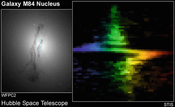
/epubstore/S/P-Schneider/Extragalactic-Astronomy-And-Cosmology/OEBPS/A129044_2_En_3_Fig41_HTML.jpg

Fig. 3.41

An HST image of the nucleus of the galaxy M84 is shown in the left-hand panel. M84 is a member of the Virgo cluster, about 15 Mpc away from us. The small rectangle depicts the position of the slit used by the STIS (Space Telescope Imaging Spectrograph) instrument on-board the HST to obtain a spectrum of the central region. The spectral shape of five emission lines, as obtained from this long-slit spectrum, is shown in the right-hand panel; the position along the slit is plotted vertically, the relative wavelength change of the light (which is proportional to the radial velocity) horizontally, also illustrated by colors. Near the center of the galaxy the wavelength suddenly changes because the rotational velocity steeply increases inwards and then changes sign on the other side of the center. This shows the Kepler rotation in the central gravitational field of a SMBH, whose mass can be estimated as $M_{\bullet } \sim 3 \times 10^{8}M_{\odot }$ . Credit: Gary Bower, Richard Green (NOAO), the STIS Instrument Definition Team, and NASA/ESA

The radius of influence. We consider a mass concentration of mass M _• in the center of a galaxy where the characteristic velocity dispersion of stars (or gas) is σ _v . We compare this velocity dispersion with the characteristic velocity (e.g., the Kepler rotational velocity) around a SMBH at a distance r, given by $\sqrt{GM_{\bullet } /r}$ . From this it follows that, for distances smaller than

$\displaystyle{ r_{\mathrm{BH}} = \frac{GM_{\bullet }} {\sigma _{v}^{2}} \sim 0.4\left ( \frac{M_{\bullet }} {10^{6}M_{\odot }}\right )\left ( \frac{\sigma _{v}} {100\,\mathrm{km/s}}\right )^{-2}\,\mathrm{pc}\;, }$

(3.44)

the SMBH will significantly affect the kinematics of stars and gas in the galaxy. The corresponding angular scale is

$\displaystyle\begin{array}{rcl} \theta _{\mathrm{BH}} = \frac{r_{\mathrm{BH}}} {D} \sim 0.\!\!^{{\prime\prime}}1\left ( \frac{M_{\bullet }} {10^{6}M_{\odot }}\right )\left ( \frac{\sigma _{v}} {100\,\mathrm{km/s}}\right )^{-2}\!\left ( \frac{D} {1\,\mathrm{Mpc}}\right )^{-1},& &{}\end{array}$

(3.45)

where D is the distance of the galaxy. From this we immediately conclude that our success in finding SMBHs will depend heavily on the achievable angular resolution. The HST enabled scientists to make huge progress in this field. The search for SMBHs promises to be successful only in relatively nearby galaxies. In addition, from (3.45) we can see that for increasing distance D the mass M _• has to increase for a SMBH to be detectable at a given angular resolution.

Kinematic evidence. The presence of a SMBH inside r _BH is revealed by an increase in the velocity dispersion for $r \lesssim r_{\mathrm{BH}}$ , which should then behave as $\sigma _{v} \propto r^{-1/2}$ for $r \lesssim r_{\mathrm{BH}}$ . If the inner region of the galaxy rotates, one expects, in addition, that the rotational velocity v _rot should also increase inwards $\propto r^{-1/2}$ .

Problems in detecting these signatures. The practical problems in observing a SMBH have already been mentioned above. One problem is the angular resolution. To measure an increase in the velocities for small radii, the angular resolution needs to be better than θ _BH. Furthermore, projection effects play a role because only the velocity dispersion of the projected stellar distribution, weighted by the luminosity of the stars, is measured. Added to this, the kinematics of stars can be rather complicated, so that the observed values for σ and v _rot depend on the distribution of orbits and on the geometry of the distribution.

Despite these difficulties, the detection of SMBHs has been achieved in recent years, largely due to the much improved angular resolution of optical telescopes (like the HST) and to improved kinematic models. Black hole masses were determined for more than 70 nearby galaxies, and upper limits on M _• were obtained for about 30 galaxies.

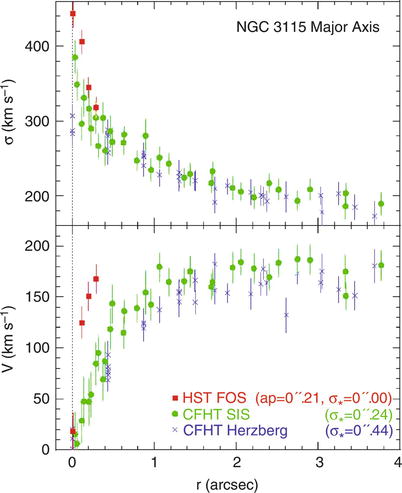
/epubstore/S/P-Schneider/Extragalactic-Astronomy-And-Cosmology/OEBPS/A129044_2_En_3_Fig42_HTML.jpg

Fig. 3.42

Rotational velocity (bottom) and velocity dispersion (top) of stars, as functions of the distance from the center along the major axis of the galaxy NGC 3115. Colors of the symbols mark observations with different instruments. Results from CFHT data which have an angular resolution of $0.\!\!^{{\prime\prime}}44$ are shown in blue. The SIS instrument at the CFHT uses active optics to achieve roughly twice this angular resolution; corresponding results are plotted in green. Finally, the red symbols show the result from HST observations using the Faint Object Spectrograph (FOS). As expected, with improved angular resolution an increase in the observed value of the velocity dispersion is detected towards the center. Even more dramatic is the impact of resolution on measurements of the rotational velocity. Due to projection effects, the measured central velocity dispersion is smaller than the real one; this effect can be corrected for. After correction, a central value of σ ∼ 600 km∕s is found. This value is much higher than the escape velocity from the central star cluster if it were to consist solely of stars—it would dissolve within ∼ 2 × 10⁴ yr. Therefore, an additional compact mass component of $M_{\bullet } \sim 10^{9}M_{\odot }$ must exist. Source: J. Kormendy & L.C. Ho 2000, Supermassive Black Holes in Inactive Galaxies, astro-ph/0003268, p. 5, Fig. 2

3.8.2 Examples for SMBHs in galaxies

Figure 3.41 shows an example for the kinematical method discussed in the previous section. A long-slit spectrum across the nucleus of the galaxy M84 clearly shows that, near the nucleus, both the rotational velocity (seen by the mean wavelength of the emission line) and the velocity dispersion (given by the width of the line) change; both increase dramatically towards the center. Figure 3.42 illustrates how strongly the measurability of the kinematical evidence for a SMBH depends on the achievable angular resolution of the observation. For this example of NGC 3115, observing with the resolution offered by space-based spectroscopy yields much higher measured velocities than is possible from the ground, due to the convolution with a larger point-spread function. Particularly interesting is the observation of the rotation curve very close to the center. Another impressive example is the central region of M87, the central galaxy of the Virgo cluster. The increase of the rotation curve and the broadening of the [Oii]-line (a spectral line of singly-ionized oxygen) at λ = 3727 Å towards the center are displayed in Fig. 3.43 and argue very convincingly for a SMBH with $M_{\bullet } \approx 3 \times 10^{9}M_{\odot }$ .

The mapping of the Kepler rotation in the center of the Seyfert galaxy NGC 4258 is especially spectacular. This galaxy contains water masers—very compact sources whose position can be observed with very high precision using VLBI techniques (Fig. 3.44). In this case, the deviation from a Kepler rotation in the gravitational field of a point mass of $M_{\bullet } \sim 3.5 \times 10^{7}M_{\odot }$ is much less than 1 %; the uncertainty in the estimated value of M _• is fully dominated by the uncertainty in the distance to this galaxy (D ∼ 7 Mpc). The maser sources are embedded in an accretion disk having a thickness of less than 0.3 % of its radius, of which also a warping is detected. Changes in the radial velocities and the proper motions of these maser sources were measured, so that the model of a Kepler accretion disk could be confirmed in detail. Several more galaxies were discovered where central masers could be used for studying the dynamics in their centers.

Hence, there are three different probes of the gravitational potential in the center of galaxies: stars, gas, and masers. All three probes are employed for identifying a SMBH in galaxies, and to determine their masses.

All these observations are of course no proof of the existence of a SMBH in these galaxies because the sources from which we obtain the kinematic evidence are still too far away from the Schwarzschild radius. The conclusion of the presence of SMBHs is rather that of a missing alternative, as was already explained for the case of the GC (Sect. 2.6.3). We have no other plausible model for the mass concentrations detected. As for the case of the SMBH in the Milky Way, an ultra-compact star cluster might be postulated, but such a cluster would not be stable over a long period of time. Moreover, its luminosity would be observed in the NIR, but there is no known stellar population that could achieve the required M∕L _NIR. Based on the existence of a SMBH in our Galaxy and in AGNs, the SMBH hypothesis is the only plausible explanation for these mass concentrations.

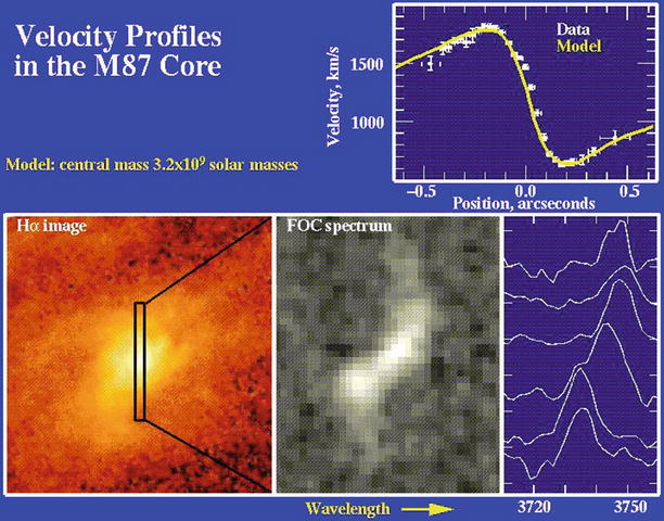
/epubstore/S/P-Schneider/Extragalactic-Astronomy-And-Cosmology/OEBPS/A129044_2_En_3_Fig43_HTML.jpg

Fig. 3.43

M87 has long been one of the most promising candidates for harboring an SMBH in its center. In this figure, the position of the slit is shown superimposed on an Hα image of the galaxy (lower left) together with the spectrum of the [Oii] line along this slit (bottom, center), and six spectra corresponding to six different positions along the slit, separated by $0.\!\!^{{\prime\prime}}14$ each (lower right). In the upper right panel the rotation curve extracted from the data using a kinematical model is displayed. These results show that a central mass concentration with $\sim 3 \times 10^{9}M_{\odot }$ must be present, confined to a region less than 3 pc across—indeed leaving basically no alternative but a SMBH. Credit: STScI, NASA, ESA, W. Keel, and Macchetto et al. 1997, ApJ 489, 579, for providing the HST FOC data

3.8.3 Correlation between SMBH mass and galaxy properties

Currently, strong indications for SMBHs have been found in the kinematics of stars or gas, resolving the sphere of influence of the black hole, in more than 70 nearby galaxies, and their masses have been estimated. This permits us to examine whether, and in what way, M _• is related to the properties of the host galaxy. In this way, a remarkable correlation was discovered: one finds that M _• is correlated with the absolute magnitude of the bulge component (or the spheroidal component) of the galaxy in which the SMBH is located (see Fig. 3.45, upper left panel). Here, the bulge component is either the bulge of a spiral or S0 galaxy or an elliptical galaxy as a whole. This correlation is described by

$\displaystyle{ M_{\bullet } = 1.7 \times 10^{9}M_{ \odot }\left ( \frac{L_{V }} {10^{11}L_{\mathrm{V}\odot }}\right )^{1.11}\;, }$

(3.46)

and indicated by the dotted line in the upper left panel of Fig. 3.45. The correlation is statistically highly significant, but the deviations of the data points from this power law are considerably larger than their error bars, with a scatter of about a factor 3 at high luminosities, increasing towards fainter galaxies. Instead of the bulge luminosity, one can also study the correlation of M _• with the mass of the bulge, which is plotted in the upper right panel of Fig. 3.45, and for which the best power-law fit

$\displaystyle{ M_{\bullet } = 2.9 \times 10^{8}M_{ \odot }\left ( \frac{M_{\mathrm{bulge}}} {10^{11}M_{\odot }}\right )^{1.05} }$

(3.47)

is obtained. For the $M_{\bullet }(M_{\mathrm{bulge}})$ relation, the scatter is slightly smaller than around the M _•(L _V ) relation. Given that the power-law index in (3.47) is almost unity, we can rewrite this relation in the form

$\displaystyle{ M_{\bullet } \approx 3 \times 10^{-3}M_{\mathrm{ bulge}}\;. }$

(3.48)

Thus we find that the black hole mass is strongly correlated with the stellar properties of the host galaxy, and that the ratio of black hole mass and bulge mass is approximately 1/300. In other words, 0.3 % of the baryon mass that was used to make the stellar population in the bulge of these galaxies was transformed into a central black hole.

/epubstore/S/P-Schneider/Extragalactic-Astronomy-And-Cosmology/OEBPS/A129044_2_En_3_Fig44_HTML.jpg

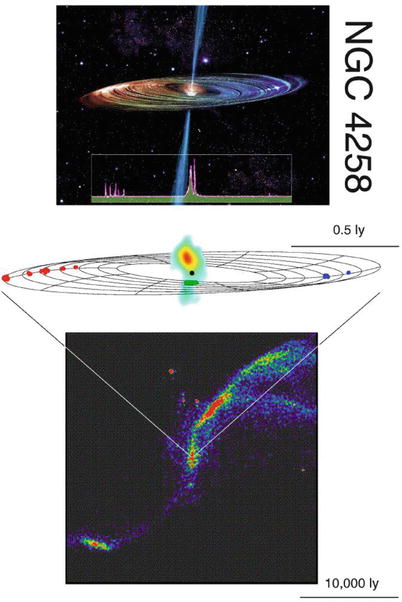
Fig. 3.44

The Seyfert galaxy NGC 4258 contains an accretion disk in its center in which several water masers are embedded. In the top image, an artist’s impression of the hidden disk and the jet is displayed, together with the line spectrum of the maser sources. Their positions (center image) and velocities have been mapped by VLBI observations. From these measurements, the Kepler law for rotation in the gravitational field of a point mass of $M_{\bullet } \sim 35 \times 10^{6}M_{\odot }$ in the center of this galaxy was verified. The best-fitting model of the central disk is also plotted. The bottom image is a 20 cm map showing the large-scale radio structure of the Seyfert galaxy. Credit: Top: M. Inoue (National Astronomical Observatory of Japan) & J. Kagaya (Hoshi No Techou). Center: Results from several groups, compiled by L. Greenhill, J. Herrnstein und J. Moran at CfA and the National Radio Astronomical Observatory. Bottom: C. De Pree, Agnes Scott College

An even tighter correlation exists between M _• and the velocity dispersion in the bulge component, as can be seen in the lower panel of Fig. 3.45. This relation is best described by

$\displaystyle{ \fbox{$M_{\bullet } = 2.1 \times 10^{8}M_{ \odot }\left ( \frac{\sigma _{v}} {200\,\mathrm{km/s}}\right )^{5.64}$}\;. }$

(3.49)

Fitting early- and late-type galaxies separately (shown by the red and blue lines in the bottom panel), the slope of the scaling relation becomes slightly flatter (5.2 and 5.06, respectively), with a normalization for the early-type galaxies being larger by about a factor 2 than that for late-type galaxies. Since the velocity dispersion in late-type galaxies is smaller than that for early-types, the difference in the normalization of the M _•(σ _v ) relation between these two galaxy populations is responsible for the steeper slope of the combined power-law fit. The scatter of the M _•(σ _v ) relation is smaller than those of the scaling relations with mass and luminosity, about a factor of ∼ 2. 5, and the scatter decreases slightly with increasing σ _v .

Hence we conclude that galaxies with a bulge component host a supermassive black hole, whose mass is tightly correlated with the properties of the stellar component; in particular, the black hole mass amounts to about 0.3 % of the stellar mass in the bulge component.

Interestingly, the black hole mass at a fixed velocity dispersion is larger by a factor ∼ 2 in early-type galaxies whose brightness profile shows a central core (see Sect. 3.2.2) than for those with a Sérsic light profile near the center.

The exact numerical coefficients in these scaling relations have been a matter of intense debate between different groups. However, these differences in the results can at least partially be traced back to different definitions of the velocity dispersion, especially concerning the choice of the spatial region across which it is measured.

There have been claims in the literature that even globular clusters contain a black hole; however, these claims are not undisputed. In addition, there may be objects that appear like globular clusters, but are in fact the stripped nucleus of a former dwarf galaxy. In this case, the presence of a central black hole is not unexpected, provided the scaling relation (3.49) holds down to very low velocity dispersion.

To date, the physical origin of this very close relation has not been understood in detail. The most obvious apparent explanation—that in the vicinity of a SMBH with a very large mass the stars are moving faster than around a smaller-mass SMBH—is not correct: the mass of the SMBH is significantly less than one percent of the mass of the bulge component. This is in contrast to the previously discussed case where the kinematics of the stars and gas were measured within the sphere of influence—but the size of this is much smaller than the bulge component itself. We can therefore disregard the contribution of the SMBH to the gravitational field in which the stars are orbiting, except in the very inner region. Instead, this correlation has to be linked to the fact that the spheroidal component of a galaxy evolves together with the SMBH. A better understanding of this relation can only be found from models of galaxy evolution. We will continue with this topic in Chap. 10.

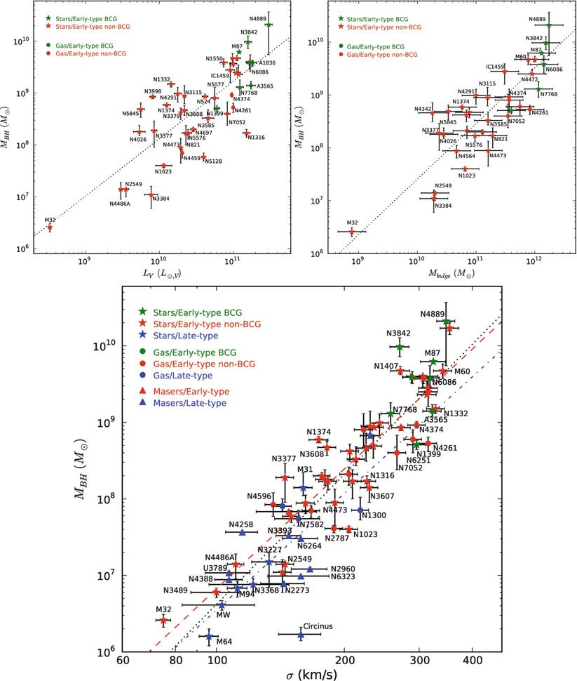
/epubstore/S/P-Schneider/Extragalactic-Astronomy-And-Cosmology/OEBPS/A129044_2_En_3_Fig45_HTML.jpg

Fig. 3.45

Black hole mass scaling relations, based on measurements of M _• in 72 nearby galaxies. The upper left panel shows M _• as a function of the optical luminosity of the bulge component for early-type galaxies with reliable photometry. In the upper right panel, M _• is plotted as a function of the bulge stellar mass, as obtained from dynamical measurements. Finally, the lower panel shows M _• versus the velocity dispersion of the spheroidal component for the full sample of 72 galaxies. Symbols indicate the methods with which M _• was determined: star-like symbols—stellar dynamics; circles—gas dynamics; triangles—masers. The color of the symbols indicate the galaxy type: green—early type brightest cluster galaxy (BCG); red—other early-type galaxies; blue—late-type galaxies. The lines in the different panels correspond to power-law fits of the various scaling relations. Source: N.J. McConnell & C.-P. Ma 2013, Revisiting the Scaling Relations of Black Hole Masses and Host Galaxy Properties, ApJ 764, 184, Figs. 1, 2 & 3. ©AAS. Reproduced with permission

3.9 Extragalactic distance determination

In Sect. 2.2 we discussed methods for distance determination within our own Galaxy. We will now proceed with the determination of distances to other galaxies. It should be noted that the Hubble law (1.2) specifies a relation between the redshift of an extragalactic object and its distance. The redshift z is easily measured from the shift in spectral lines. For this reason, the Hubble law (and its generalization—see Sect. 4.3.3) provides a simple method for determining distance. However, to apply this law, first the Hubble constant H ₀ must be known, i.e., the Hubble law must be calibrated. Therefore, in order to determine the Hubble constant, distances have to be measured independently from redshift.

Peculiar motions. Furthermore, it has to be kept in mind that besides the general cosmic expansion, which is expressed in the Hubble law, objects also show peculiar motion, like the velocities of galaxies in clusters of galaxies or the motion of the Magellanic Clouds around our Milky Way. These peculiar velocities are induced by gravitational acceleration resulting from the locally inhomogeneous mass distribution in the Universe. For instance, our Galaxy is moving towards the Virgo cluster of galaxies, a dense accumulation of galaxies, due to the gravitational attraction caused by the cluster mass, and our neighboring galaxy M31 is actually approaching us because of mutual gravitational attraction. The measured redshift, and therefore the Doppler shift, is always a superposition of the cosmic expansion velocity and peculiar velocities.

CMB dipole anisotropy. The peculiar velocity of the Galaxy is very precisely known. The radiation of the cosmic microwave background is not completely isotropic but instead shows a dipole component. This component originates in the velocity of the Solar System relative to the rest frame in which the CMB appears isotropic (see Fig. 1.21). Due to the Doppler effect, the CMB appears hotter than average in the direction of our motion and cooler in the opposite direction. Analyzing this CMB dipole allows us to determine our peculiar velocity, which yields the result that the Sun moves at a velocity of (368 ± 2) km∕s relative to the CMB rest frame. Furthermore, the Local Group of galaxies (see Sect. 6.1) is moving at $v_{\mathrm{LG}} \approx 600\,\mathrm{km/s}$ relative to the CMB rest frame.

/epubstore/S/P-Schneider/Extragalactic-Astronomy-And-Cosmology/OEBPS/A129044_2_En_3_Fig46_HTML.jpg

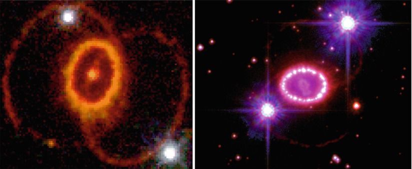
Fig. 3.46

Left panel: The ring around supernova 1987A in the LMC, as seen 7 years after the explosion, is illuminated by photons from the explosion which induce the radiation from the gas in the ring. It is inclined towards the line-of-sight; thus it appears to be elliptical. Lighting up of the ring was not instantaneous, due to the finite speed of light: those sections of the ring closer to us lit up earlier than the more distant parts. From the time shift in the onset of radiation across the ring, its diameter can be derived. Combining this with the measured angular diameter of the ring, the distance to SN 1987A—and thus the distance to the LMC—can be determined. The picture on the right shows an image of the ring, taken with the HST about 20 years after the original explosion (and with a different orientation of the telescope). In this later image, the ring is seen to host a large number of bright spots, which were not observed in the earlier image seen on the left. These bright spots correspond to gas concentrations in the inner regions of the ring, which were heated up, and thus exited to glow, by the supernova blast wave slamming into the ring. Since the blast wave propagates with a velocity much smaller than c, it took about 10 years before it reached the innermost parts of the ring and the first spots were seen. The material seen inside the ring is debris from the explosion, heated up by radioactive decays of nuclei which were formed during the supernova. Credit: NASA, STScI, ESA, P. Challis and R. Kirshner (Harvard-Smithsonian Center for Astrophysics)

Distance ladder. For the redshift of a source to be dominated by the Hubble expansion, the cosmic expansion velocity $v = cz = H_{0}D$ has to be much larger than typical peculiar velocities. This means that in order to determine H ₀ we have to consider sources at large distances for the peculiar velocities to be negligible compared to H ₀ D.

Direct estimates of the distances of distant galaxies are very difficult to obtain. Traditionally one uses a distance ladder: at first, the absolute distances to nearby galaxies are measured directly. If methods to measure relative distances (that is, distance ratios) with sufficient precision are utilized, the distances to galaxies further away are then determined relative to those nearby. In this way, by means of relative methods, distances are estimated for galaxies that are sufficiently far away so that their redshifts are dominated by the Hubble flow.

3.9.1 Distance of the LMC

The distance of the Large Magellanic Cloud (LMC) can be estimated using various methods. For example, we can resolve and observe individual stars in the LMC, which forms the basis of the MACHO experiments (see Sect. 2.5.2). Because the metallicity of the LMC is significantly lower than that of the Milky Way, some of the methods discussed in Sect. 2.2 are only applicable after correcting for metallicity effects, e.g., the photometric distance determination or the period-luminosity relation for pulsating stars.

Supernova 1987A. Perhaps the most precise method of determining the distance to the LMC is a purely geometrical one. The supernova SN 1987A that exploded in 1987 in the LMC illuminates a nearly perfectly elliptical ring (see Fig. 3.46). This ring consists of material that was once ejected by the stellar winds of the progenitor star of the supernova and that is now radiatively excited by energetic photons from the supernova explosion. The corresponding recombination radiation is thus emitted only when photons from the SN hit the surrounding gas. Because the observed ring is almost certainly intrinsically circular and the observed ellipticity is caused only by its inclination with respect to the line-of-sight, the distance to SN 1987A can be derived from observations of the ring. First, the inclination angle is determined from its observed ellipticity. The gas in the ring is excited by photons from the SN a time R∕c after the original explosion, where R is the radius of the ring. We do not observe the illumination of the ring instantaneously because light from the section of the ring closer to us reaches us earlier than light from the more distant part. Thus, its illumination was seen sequentially along the ring. Combining the time delay in the illumination between the nearest and farthest part of the ring with its inclination angle, we then obtain the physical diameter of the ring. When this is compared to the measured angular size of the major axis of $\sim 1.\!\!^{{\prime\prime}}7$ , the ratio yields the distance to SN 1987A,

$\displaystyle{D_{\mathrm{SN1987A}} \approx 51.8\,\mathrm{kpc} \pm 6\%\;.}$

If we now assume the extent of the LMC along the line-of-sight to be small, this distance can be identified with the distance to the LMC. The value is also compatible with other distance estimates (e.g., as derived by using photometric methods based on the properties of main sequence stars—see Sect. 2.2.4).

Most recently, the distance to the LMC was determined by observing eclipsing binary systems with a long orbital period. Spectroscopy allowed the accurate determination of the orbits of these systems, which together with the measured angular separation yielded the distances to these binaries. This resulted in a distance to the LMC of

$\displaystyle{D_{\mathrm{EB}} = 50.0\,\mathrm{kpc} \pm 2.2\%\;.}$

3.9.2 The Cepheid distance

In Sect. 2.2.7, we discussed the period-luminosity relation of pulsating stars. Due to their high luminosity, Cepheids turn out to be particularly useful since they can be observed out to large distances.

For the period-luminosity relation of the Cepheids (also called the Leavitt law) to be a good distance measure, it must first be calibrated. This calibration has to be done with as large a sample of Cepheids as possible at a known distance. Cepheids in the LMC are well-suited for this purpose because we believe we know the distance to the LMC quite precisely, see above. Also, due to the relatively small extent of the LMC along the line-of-sight, all Cepheids in the LMC should be located at approximately the same distance. For this reason, the period-luminosity relation is calibrated using the Cepheids in the LMC. Due to the large number of Cepheids available for this purpose (several thousands, many of which were found in the microlens surveys discussed in Sect. 2.5.3), the resulting statistical errors are small. However, uncertainties remain in the form of systematic errors related to the metallicity dependence of the period-luminosity relation, as well as with regards to interstellar extinction. These effects can be corrected for since the color of Cepheids depends on the metallicity as well.

With the high angular resolution of the HST, individual Cepheids in galaxies are visible at distances up to that of the Virgo cluster of galaxies. In fact, determining the distance to Virgo as a central step in the determination of the Hubble constant was one of the major scientific aims of the HST. In the Hubble Key Project , the distances to numerous spiral galaxies in the Virgo cluster were determined by identifying Cepheids and measuring their periods.

Since most of the galaxies for which these Cepheid distances were determined have a metallicity that is comparable to that of the Milky Way, rather than the LMC, the aforementioned metallicity effects, as well as the absolute distance determination to the LMC, remained the main source of systematic uncertainty in the determination of galaxy distances in the Virgo cluster. Over the past few years, these uncertainties could be reduced substantially by measuring the trigonometric parallaxes of ten Galactic Cepheids at distances between 300 pc and 600 pc with the HST. This allowed a calibration of the period-luminosity relation with an accuracy of about 3 %. Since the number of these Galactic Cepheids is still rather small, and all but one have periods below 10 days, one can use the slope of the period-luminosity as obtained from LMC Cepheids, where the statistics is much better, but determine the amplitude of this relation from the Galactic Cepheids.

Another way to accurately calibrate Cepheid distances is provided by the maser galaxy NGC 4258 (Fig. 3.44) mentioned before. The dynamics of the maser source can be studied with great accuracy, due to the compact nature of these source, and these results can be interpreted straightforwardly, due to the simple orbital motion of the sources. In particular, with measurements of proper motions and acceleration of the maser sources in a Keplerian disk, the distance to NGC 4258 could be determined to be D = 7. 2 ± 0. 2 Mpc. This distance estimate can then be used to calibrate the period-luminosity relation from Cepheids in this galaxy.

With these new results, the calibration of Cepheid distances has been considerably improved relative to that based on LMC Cepheids alone. It should also be noted that the new period-luminosity relation does not depend on the adopted distance to the LMC anymore. Conversely, with the newly calibrated period-luminosity relation, the distance to the LMC can be determined, yielding $D_{\mathrm{LMC}} = 47.9\,\mathrm{kpc}$ , with an estimated error of ∼ 3 %.

3.9.3 Tip of the Red Giant Branch

Another method which can be used to determine the distance to nearby galaxies is based on the color-magnitude relation of red giant branch stars. This method is based on the fact that red giant stars have a maximum luminosity, as is well understood from the theory of stellar evolution.⁸ This maximum luminosity, which depends on the laws of nuclear physics, is almost independent of the chemical composition of a star. It can be identified by a clear discontinuity in the number of red giants in a galaxy as a function of magnitude. Relating the apparent magnitude of this tip of the red giant branch in a galaxy to the known absolute magnitude of this maximum luminosity, the distance to the galaxy can be determined.

Whereas red giants are less luminous that Cepheids, and thus cannot be observed to equally large distances, the tip of the red giant branch method can still be used for galaxies as far away as the Virgo cluster. Therefore, this method serves as a calibration for galaxy distances, independent of the Cepheid method.

3.9.4 Supernovae Type Ia

As mentioned in Sect. 2.3.2, according to the (arguably) most plausible model, Type Ia supernovae are supposed to be the result of explosion processes of white dwarfs which cross a critical mass threshold by accretion of additional matter. This threshold should be identical for all SNe Ia, making it at least plausible that they all have the same luminosity. If this were the case, they would be ideal for standard candles: owing to their high luminosity, they can be detected and examined even at very large distances.

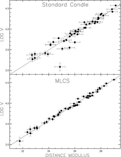
/epubstore/S/P-Schneider/Extragalactic-Astronomy-And-Cosmology/OEBPS/A129044_2_En_3_Fig47_HTML.jpg

Fig. 3.47

The Hubble diagram for relatively nearby SNe Ia. Plotted is the measured expansion velocity cz as a function of the distance modulus for the individual supernovae. In the top panel, it is assumed that all sources have the same luminosity. If this was correct, all data points should be aligned along the straight line, as follows from the Hubble law. Obviously, the scatter is significant. In the bottom panel, the luminosities have been corrected by means of the so-called MLCS method in which the shape of the light curve and the colors of the SN are used to ‘standardize’ the luminosity (see text for more explanations). By this the deviations from the Hubble law become dramatically smaller—the dispersion is reduced from 0. 42 to 0. 15 mag. Source: A.V. Filippenko & A.G. Riess 2000, Evidence from Type Ia Supernovae for an Accelerating Universe, astro-ph/0008057, p. 5, Fig. 1

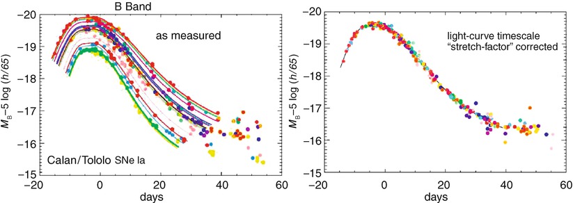
/epubstore/S/P-Schneider/Extragalactic-Astronomy-And-Cosmology/OEBPS/A129044_2_En_3_Fig48_HTML.jpg

Fig. 3.48

Left panel: B-band light curves of different SNe Ia. One sees that the shape of the light curves and the maximum luminosity of the SNe Ia differ substantially among the sample. A transformation was found empirically with a single parameter described by the width of the light curve. By means of this transformation, the different light curves can all be made congruent, as displayed in the right panel. Credit: M. Hamuy, S. Perlmutter, Supernova Cosmology Project

However, it turns out that SNe Ia are not really standard candles, since their maximum luminosity varies from object to object with a dispersion of about 0. 4 mag in the blue band light. This is visible in the top panel of Fig. 3.47. If SNe Ia were standard candles, the data points would all be located on a straight line, as described by the Hubble law. Clearly, deviations from the Hubble law can be seen, which are significantly larger than the photometric measurement errors.

It turns out that there is a strong correlation between the luminosity and the shape of the light curve of SNe Ia. Those of higher maximum luminosity show a slower decline in the light curve, as measured from its maximum. Furthermore, the observed flux is possibly affected by extinction in the host galaxy, in addition to the extinction in the Milky Way. With the resulting reddening of the spectral distribution, this effect can be derived from the observed colors of the SN. The combined analysis of these effects provides a possibility for deducing an empirical correction to the maximum luminosity from the observed light curves in several filters, accounting both for the relation of the width of the curve to the observed luminosity and for the extinction. This correction was calibrated on a sample of SNe Ia for which the distance to the host galaxies is very accurately known.⁹ With this correction applied, the SNe Ia follow the Hubble law much more closely, as can be seen in the bottom panel of Fig. 3.47. A scatter of only σ = 0. 15 mag around the Hubble relation remains. Figure 3.48 demonstrates the effect of this correction on the light curves of several SNe Ia which initially appear to have very different maximum luminosities and widths. After correction they become nearly identical. The left panel of Fig. 3.48 suggests that the light curves of SN Ia can basically be described by a one-parameter family of functions, and that this parameter can be deduced from the shape, in particular the width, of the light curves.

With this correction, SNe Ia become standardized candles, i.e., by observing the light curves in several bands their ‘corrected’ maximum luminosity can be determined. Since the observed flux of a source depends on its luminosity and its distance, once the luminosity is known and the flux measured, the distance to the SN Ia can be inferred. SNe Ia are visible out to very large distances, so that they also permit distance estimates at such large redshifts where the simple Hubble law (1.6) is no longer valid, but needs to be generalized based on a cosmological model (Sect. 4.3.3). We will see in Sect. 8.3 that these measurements belong to the most important pillars on which our standard model of cosmology rests.

3.9.5 Secondary distance indicators

The Virgo cluster, at a measured distance of about 16 Mpc, is not sufficiently far away from us to directly determine the Hubble constant from its distance and redshift, because peculiar velocities still contribute considerably to the measured redshift at this distance. To get to larger distances, a number of relative distance indicators are used. They are all based on measuring the distance ratio of galaxies. If the distance to one of the two is known, the distance to the other is then obtained from the ratio. By this procedure, distances to more remote galaxies can be measured. Below, we will review some of the most important secondary distance indicators.

Surface brightness fluctuations of galaxies. Another method of estimating distance ratios is surface brightness fluctuations. It is based on the fact that the number of bright stars per area element in a galaxy fluctuates—purely by Poisson noise: If N stars are expected in an area element, the relative fluctuations of the number of stars will be $\sqrt{N}/N = 1/\sqrt{N}$ . These fluctuation in the number of stars are observed as fluctuations of the local surface brightness. To demonstrate that this effect can be used to estimate distances, we consider a solid angle dω. The corresponding area element dA = D ² dω depends quadratically on the distance D of the galaxy. If we now consider two galaxies at a radius from their center where their surface brightnesses are the same,¹⁰ and assume that their stellar populations are comparable, then the galaxy with the larger distance from us will have a larger the number of stars N in this solid angle. Correspondingly, its relative fluctuations of the surface brightness will be smaller. By comparing the surface brightness fluctuations of different galaxies, one can therefore estimate relative distances. This method also has to be calibrated on the galaxies for which Cepheid or other primary distances are available.

Planetary nebulae. The brightness distribution of planetary nebulae in a galaxy seems to have an upper limit which is the nearly the same for each galaxy (see Fig. 3.49). If a sufficient number of planetary nebulae are observed and their brightnesses measured, it enables us to determine their luminosity function from which the maximum apparent magnitude is then derived. By calibration on galaxies of known Cepheid distance, the corresponding maximum absolute magnitude can be determined, which then allows the determination of the distance modulus for other galaxies, thus their distances.

Scaling relations. The scaling relations for galaxies—fundamental plane for ellipticals, Tully–Fisher relation for spirals (see Sect. 3.4)—can be calibrated on local groups of galaxies or on the Virgo cluster, the distances of which have been determined from Cepheids. Although the scatter of these scaling relations can be 15 % for individual galaxies, the statistical fluctuations are reduced when observing several galaxies at about the same distance (such as in clusters and groups). This enables us to estimate the distance ratio of two clusters of galaxies.

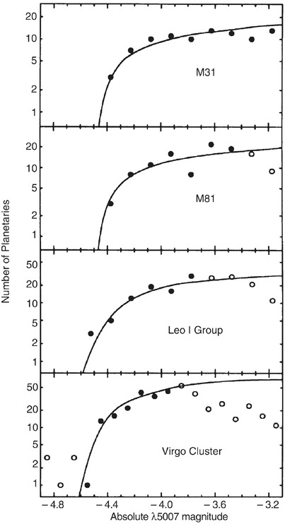
/epubstore/S/P-Schneider/Extragalactic-Astronomy-And-Cosmology/OEBPS/A129044_2_En_3_Fig49_HTML.jpg

Fig. 3.49

Brightness distribution of planetary nebulae in Andromeda (M31), M81, three galaxies in the Leo I group, and six galaxies in the Virgo cluster. The plotted absolute magnitude was measured in the emission line of double-ionized oxygen at λ = 5007 Å in which a large fraction of the luminosity of a planetary nebula is emitted. This characteristic line emission is also used in the identification of such objects in other galaxies. In all cases, the distribution is described by a nearly identical luminosity function; it seems to be a universal function in galaxies. Therefore, the brightness distribution of planetary nebulae can be used to estimate the distance of a galaxy. In the fits shown, the data points marked by open symbols were disregarded: at these magnitudes, the distribution function is probably not complete. Source: G.H. Jacoby et al. 1992, A critical review of selected techniques for measuring extragalactic distances, PASP 104, 599, p. 635, Fig. 15

3.9.6 The Hubble Constant

Using the various methods described above, the Hubble Key Project aimed at determining the value of the Hubble constant. Cepheid distances to 18 galaxies in the range $3\,\mathrm{Mpc} \leq D \leq 25\,\mathrm{Mpc}$ were determined, which were then used to calibrate the Tully–Fischer relation for spirals, the D _n −σ relation for ellipticals, the peak luminosity of SN Ia, and the surface brightness fluctuation method. These secondary distance indicators were then applied to galaxies as much larger distances, such that their peculiar velocity is negligible compared to their radial velocity according to the Hubble law.

By combining the various methods, a distance to the Coma cluster of about 90 Mpc was obtained. Furthermore, using the SN Ia technique, distances of galaxies with $D \lesssim 400\,\mathrm{Mpc}$ could be measured. The resulting Hubble constant, incorporating the new calibration of the period-luminosity relation from Cepheids in the Milky Way and in NGC 4258, reads

$\displaystyle{ \fbox{$H_{0} = 74 \pm 3\,\mathrm{km/s/Mpc}$}\;. }$

(3.50)

The error given here denotes the estimated systematic uncertainty in the determination of H ₀, whereas the statistical uncertainty is smaller by a factor of two and thus subdominant. Thus, the dimensionless Hubble constant, defined in (1.7), is h = 0. 74 ± 0. 03. A convenient way to memorize this is h ² ≈ 1∕2.

Thus, the uncertainty about the value of the Hubble constant has finally shrunk to a mere 6 %—after decades of intense debates between two camps of scientists, where the first camp obtained values near $50\,\mathrm{km/s/Mpc}$ , and the other camp about twice this value, each with error bars that were very much smaller than the differences between their results.

We will see later that the Hubble constant can also be measured by completely different methods. The currently most accurate of these, based on tiny small-scale anisotropies of the cosmic microwave background (Sect. 8.7.1), results in a value which is in fairly good agreement with that in (3.50), and yields a smaller estimated error.

3.10 Luminosity function of galaxies

Definition of the luminosity function. The luminosity function specifies the way in which the members of a class of objects are distributed with respect to their luminosity. More precisely, the luminosity function is the number density of objects (here galaxies) of a specific luminosity. Φ(M) dM is defined as the number density of galaxies with absolute magnitude in the interval [M, M + dM]. The total density of galaxies is then

$\displaystyle{ \nu =\int _{ -\infty }^{\infty }\mathrm{d}M\;\varPhi (M)\;. }$

(3.51)

Accordingly, Φ(L) dL is defined as the number density of galaxies with a luminosity between L and L + dL. It should be noted here explicitly that both definitions of the luminosity function are denoted by the same symbol, although they represent different mathematical functions, i.e., they describe different functional relations. It is therefore important (and in most cases not difficult) to deduce from the context which of these two functions is being referred to.

Problems in determining the luminosity function. At first sight, the task of determining the luminosity function of galaxies does not seem very difficult. The history of this topic shows, however, that we encounter a number of problems in practice. As a first step, the determination of galaxy luminosities is required, for which, besides measuring the flux, distance estimates are also necessary. For very distant galaxies redshift is a sufficiently reliable measure of distance, whereas for nearby galaxies the methods discussed in Sect. 3.9 have to be applied.

Another problem occurs for nearby galaxies, namely the large-scale structure of the galaxy distribution. To obtain a representative sample of galaxies, a sufficiently large volume has to be surveyed because the galaxy distribution is heavily structured on scales of ∼ 100h ⁻¹ Mpc and more. On the other hand, galaxies of particularly low luminosity can only be observed locally, so the determination of Φ(L) for small L always needs to refer to local galaxies. Finally, one has to deal with the so-called Malmquist bias; in a flux-limited sample luminous galaxies will always be overrepresented because they are visible at larger distances (and therefore are selected from a larger volume). A correction for this effect is always necessary, and was applied, e.g., to Fig. 3.7.

3.10.1 The Schechter luminosity function

The global galaxy distribution can be roughly approximated by the Schechter luminosity function

$\displaystyle{ \fbox{$\varPhi (L) = \left ( \frac{\varPhi ^{{\ast}}} {L^{{\ast}}}\right )\,\left ( \frac{L} {L^{{\ast}}}\right )^{\alpha }\,\exp \left (-L/L^{{\ast}}\right )$}\;, }$

(3.52)

where L ^∗ is a characteristic luminosity above which the distribution decreases exponentially, α is the slope of the luminosity function for small L, and Φ ^∗ specifies the normalization of the distribution. A schematic plot of this function, as well as a fit to early data, is shown in Fig. 3.50.

/epubstore/S/P-Schneider/Extragalactic-Astronomy-And-Cosmology/OEBPS/A129044_2_En_3_Fig50_HTML.jpg

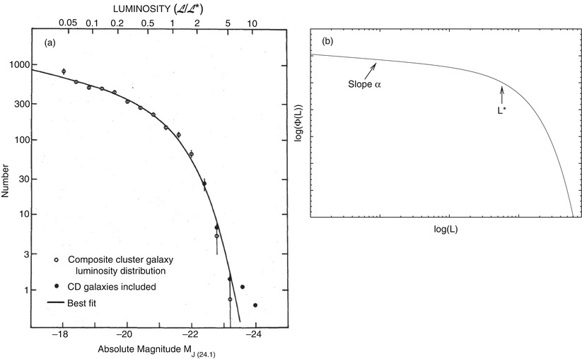
Fig. 3.50

Left panel: galaxy luminosity function as obtained from 13 clusters of galaxies. For the solid circles, cD galaxies have also been included. Right panel: a schematic plot of the Schechter function. Source (left panel): P. Schechter 1976, An analytic expression for the luminosity function for galaxies, ApJ 203, 297, p. 300, Fig. 2. ©AAS. Reproduced with permission

Expressed in magnitudes, this function appears much more complicated. Considering that an interval dL in luminosity corresponds to an interval dM in absolute magnitude, with $\mathrm{d}L/L = -0.4\,\ln 10\,\mathrm{d}M$ , and using $\varPhi (L)\,\mathrm{d}L =\varPhi (M)\,\mathrm{d}M$ , i.e., the number of sources in these intervals are of course the same, we obtain

$\displaystyle\begin{array}{rcl} \varPhi (M)& =& \varPhi (L)\,\left \vert \frac{\mathrm{d}L} {\mathrm{d}M}\right \vert =\varPhi (L)\,0.4\,\ln 10\,L{}\end{array}$

(3.53)

$\displaystyle\begin{array}{rcl} & =& 0.921\varPhi ^{{\ast}}10^{0.4(\alpha +1)(M^{{\ast}}-M) }\exp \left (-10^{0.4(M^{{\ast}}-M) }\right )\;.{}\end{array}$

(3.54)

As mentioned above, the determination of the parameters entering the Schechter function is difficult; a characteristic set of parameters in the blue band is given as

$\displaystyle\begin{array}{rcl} \varPhi ^{{\ast}}& =& 1.6 \times 10^{-2}h^{3}\,\mathrm{Mpc}^{-3}\;, \\ M_{B}^{{\ast}}& =& -19.7 + 5\log h\quad \mathrm{or} \\ L_{B}^{{\ast}}& =& 1.2 \times 10^{10}h^{-2}L_{ \odot,\mathrm{B}}\;, \\ \alpha & =& -1.07\;. {}\end{array}$

(3.55)

While the blue light of galaxies can be strongly affected by star formation, the luminosity function in the red bands measures the typical stellar distribution. In the K-band, we have

$\displaystyle\begin{array}{rcl} \varPhi ^{{\ast}}& =& 1.6 \times 10^{-2}h^{3}\,\mathrm{Mpc}^{-3}\;, \\ M_{K}^{{\ast}}& =& -23.1 + 5\log h\;, \\ \alpha & =& -0.9\;. {}\end{array}$

(3.56)

The total number density of galaxies is formally infinite if α ≤ −1, but the validity of the Schechter function does of course not extend to arbitrarily small L. The luminosity density¹¹

$\displaystyle{ l_{\mathrm{tot}} =\int _{ 0}^{\infty }\mathrm{d}L\;L\,\varPhi (L) =\varPhi ^{{\ast}}\,L^{{\ast}}\,\varGamma (2+\alpha ) }$

(3.58)

is finite for α ≥ −2. The integral in (3.58), for α ∼ −1, is dominated by L ∼ L ^∗, and n = Φ ^∗ is thus a good estimate for the mean density of L ^∗-galaxies.

In fact, whereas the rise of the Schechter luminosity function towards small L may at first sight suggest that low-L galaxies are ‘more important’ than higher luminosity objects, this is clearly not the case. Quite the contrary: for $\alpha = -1$ , 60 % of the whole luminosity of the galaxy population is emitted from objects with $0.22L^{{\ast}}\leq L \leq 1.6L^{{\ast}}$ , and 90 % of the luminosity stems from galaxies with $0.1 \leq L/L^{{\ast}}\leq 2.3$ . Hence, the total luminosity of galaxies stems from a fairly narrow range around ∼ L ^∗∕2. Since the luminosity, specifically in red and NIR bands, is almost proportional to the stellar mass, most of the stars in the Universe live in ∼ L ^∗ -galaxies. The parameters of the Schechter function then tell us that the mean number density of ‘typical’ galaxies (i.e., those with L ∼ L ^∗) is about $2 \times 10^{-2}h^{3}\,\mathrm{Mpc}^{-3}$ , meaning that the mean separation between two luminous galaxies is about $4h^{-1}\,\mathrm{Mpc}$ .

Fig. 3.51

The luminosity function for different Hubble types of field galaxies (top) and galaxies in the Virgo cluster of galaxies (bottom). Dashed curves denote extrapolations. In contrast to Fig. 3.50, the more luminous galaxies are plotted towards the left. The Schechter luminosity function of the total galaxy distribution is the sum of the luminosity functions of individual galaxy types which can deviate significantly from the Schechter function. One can see that in clusters the major contribution at faint magnitudes comes from the dwarf ellipticals (dEs), and that at the bright end ellipticals and S0s contribute much more strongly to the luminosity function than they do in the field. This trend is even more prominent in regular clusters of galaxies. Source: B. Binggeli et al. 1988, The luminosity function of galaxies, ARA&A 26, 509, Fig. 1, p. 542. Reprinted, with permission, from the Annual Review of Astronomy & Astrophysics, Volume 26 ©1988 by Annual Reviews www.annualreviews.org

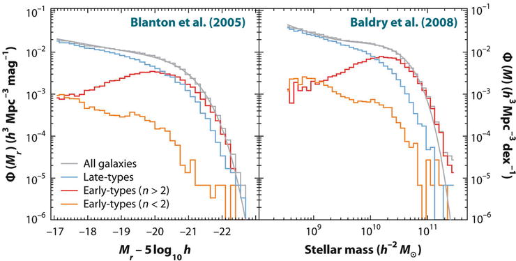
/epubstore/S/P-Schneider/Extragalactic-Astronomy-And-Cosmology/OEBPS/A129044_2_En_3_Fig52_HTML.jpg

Fig. 3.52

Left panel: The luminosity function of galaxies, i.e., the number density of galaxies as a function of absolute r-band magnitude. The total luminosity function is shown as the grey histogram, with the smooth curve being a fit with a double-Schechter function (3.59). Also shown are the luminosity function of early-type galaxies, split according to the Sérsic index n into concentrated and less concentrated ones (red and orange histograms, respectively), and late-type galaxies shown in blue. The early-types with n ≤ 2 are totally subdominant for all L, and contribute substantially to the early-type population only for very low luminosities, in agreement with what is seen in Fig. 3.39. Right panel: The stellar mass function of galaxies, with the same galaxy populations as in the left-hand panel. The total mass function is again fit with a double-Schechter function. Source: M.R. Blanton & J. Moustakas 2009, Physical Properties and Environments of Nearby Galaxies, ARA&A 47, 159, p. 166, Fig. 3. Reprinted, with permission, from the Annual Review of Astronomy & Astrophysics, Volume 47 ©2009 by Annual Reviews www.annualreviews.org

3.10.2 More accurate luminosity and mass functions

With better statistics of galaxy surveys, it became clear that the luminosity function of galaxies deviates from the Schechter form. There is also no obvious reason why such a simple relation for describing the luminosity distribution of galaxies should exist. Whereas the Schechter function approximates the total galaxy distribution, each morphological type of galaxy has its own luminosity function, with a shape that can significantly deviate from a Schechter function—see Fig. 3.51. For instance, spirals are relatively narrowly distributed in L, whereas the distribution of ellipticals is much broader if we account for the full L-range, from giant ellipticals to dwarf ellipticals, although, if we just consider normal ellipticals, their luminosity range is comparable to that of spirals. Ellipticals dominate in particular at large L; the low end of the luminosity function is likewise dominated by dwarf ellipticals and irregular galaxies. In addition, the luminosity distribution of cluster and group galaxies differs from that of field galaxies. The fact that these populations add up to something as simple as (3.52) is a most likely a coincidence.

Indeed, the size and quality of the Sloan Digital Sky Survey and other redshift surveys allowed more robust conclusions about the luminosity function of galaxies. For the total population, a good fit is obtained by using a double-Schechter function of the form

$\displaystyle\begin{array}{rcl} \varPhi (L)& =& \left [\left ({ \varPhi _{1}^{{\ast}} \over L^{{\ast}}}\right )\,\left ({ L \over L^{{\ast}}}\right )^{\alpha _{1}} + \left ({ \varPhi _{2}^{{\ast}} \over L^{{\ast}}}\right )\,\left ({ L \over L^{{\ast}}}\right )^{\alpha _{2}}\right ] \\ & & \times \exp \left (-L/L^{{\ast}}\right )\;, {}\end{array}$

(3.59)

with two normalizations Φ _i ^∗ and two slopes α _i , but the same cut-off luminosity L ^∗. This form allows a transition of the slope of the luminosity function, which for very small L is given by the more negative ones of the two α’s. In Fig. 3.52, we show the r-band luminosity function of nearby galaxies as obtained from the SDSS, separated into galaxy types, together with a double-Schechter fit to the total galaxy population. At the luminous end of the distribution, early-type galaxies dominate the luminosity function, although not by a large factor. For faint galaxies, the situation is reversed, with late-type galaxies being much more numerous than early types. This is due to the fact that the slope of the faint-end luminosity function is much steeper for late-type galaxies. If we consider instead the luminosity function in the near ultraviolet, it is totally dominated by late-type galaxies at all L.

Interestingly, the value of L ^∗ in the double Schechter function is the same for the two components—one might have expected that a better fit could be obtained by the sum of two Schechter functions, with two different values of the cut-off luminosity L ^∗. This, however, is not the case. It thus seems that L ^∗ corresponds to a characteristic luminosity of galaxies, whose value is fixed by the physics of galaxy formation and evolution. As we will show in Chap. 10, this is indeed the case.

The right-hand panel of Fig. 3.52 displays the corresponding mass function of galaxies, obtained from the luminosity function using the appropriate M∕L for the stellar population. Here we see that the dominance of early-type galaxies at the high stellar mass end of the distribution is even stronger, since they have a higher M∕L than late types.

The mass functions of individual galaxy types can be used to estimate where most of the stellar mass is located. Curiously, about one third of the stellar mass is contained in disks, one third in ellipticals, and one third in bulges and bars.

3.11 Galaxies as gravitational lenses

In Sect. 2.5 the gravitational lens effect was discussed, where we concentrated on the deflection of light by point masses. The lensing effect by stars leads to image separations too small to be resolved by any existing telescope. Since the separation angle is proportional to the square root of the lens mass (2.82), the angular separation of the images will be about a million times larger if a galaxy acts as a gravitational lens. In this case it should be observable, as was predicted in 1937 by Fritz Zwicky. Indeed, multiple images of very distant sources have been found, together with the galaxy responsible for the image splitting. In this section we will first describe this effect by continuing the discussion we began in Sect. 2.5.1. Examples of the lens effect and its various applications will then be discussed.

3.11.1 The gravitational lens effect—Part II

The geometry of a typical gravitational lens system is sketched in Fig. 2.30 and again in Fig. 3.53. The physical description of such a lens system for an arbitrary mass distribution of the deflector is obtained from the following considerations.

If the gravitational field is weak (which is the case in all situations considered here), the gravitational effects can be linearized.¹² Hence, the deflection angle of a lens that consists of several mass components can be described by a linear superposition of the deflection angles of the individual components,

$\displaystyle{ \hat{{\boldsymbol \alpha }}=\sum _{i}\hat{{\boldsymbol \alpha }}_{i}\;. }$

(3.60)

We assume that the deflecting mass has a small extent along the line-of-sight, as compared to the distances between observer and lens (D _d) and between lens and source (D _ds). All mass elements can then be assumed to be located at the same distance D _d. This physical situation is called a geometrically thin lens. If a galaxy acts as the lens, this condition is certainly fulfilled—the extent of galaxies is typically $\sim 100h^{-1}\,\mathrm{kpc}$ while the distances of lens and source are typically ∼ Gpc. We can therefore write (3.60) as a superposition of Einstein angles of the form (2.74),

$\displaystyle{ \hat{{\boldsymbol \alpha }}({\boldsymbol \xi }) =\sum _{i}\frac{4Gm_{i}} {c^{2}} \frac{{\boldsymbol \xi }-{\boldsymbol \xi }_{i}} {\left \vert {\boldsymbol \xi }-{\boldsymbol \xi }_{i}\right \vert ^{2}}\;, }$

(3.61)

where ${\boldsymbol \xi }_{i}$ is the projected position vector of the mass element m _i , and ${\boldsymbol \xi }$ describes the position of the light ray in the lens plane, also called the impact vector.

/epubstore/S/P-Schneider/Extragalactic-Astronomy-And-Cosmology/OEBPS/A129044_2_En_3_Fig53_HTML.jpg

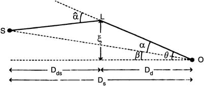
Fig. 3.53

As a reminder, another sketch of the lens geometry. Source: R.D. Blandford & R. Narayan 1992, Cosmological applications of gravitational lensing, ARA&A 30, 311, Fig. 5, p. 318. Reprinted, with permission, from the Annual Review of Astronomy & Astrophysics, Volume 30 ©1992 by Annual Reviews www.annualreviews.org

For a continuous mass distribution we can imagine subdividing the lens into mass elements of mass $\mathrm{d}m =\varSigma ({\boldsymbol \xi })\,\mathrm{d}^{2}\xi$ , where $\varSigma ({\boldsymbol \xi })$ describes the surface mass density of the lens at the position ${\boldsymbol \xi }$ , obtained by projecting the spatial (three-dimensional) mass density ρ along the line-of-sight to the lens. With this definition the deflection angle (3.61) can be transformed into an integral,

$\displaystyle{ \fbox{$\hat{{\boldsymbol \alpha }}({\boldsymbol \xi }) = \frac{4G} {c^{2}} \int \mathrm{d}^{2}\xi '\;\varSigma ({\boldsymbol \xi }') \frac{{\boldsymbol \xi }-{\boldsymbol \xi }'} {\left \vert {\boldsymbol \xi }-{\boldsymbol \xi }'\right \vert ^{2}}$}\;. }$

(3.62)

This deflection angle is then inserted into the lens equation (2.78),

$\displaystyle{ {\boldsymbol \beta }={\boldsymbol \theta } -\frac{D_{\mathrm{ds}}} {D_{\mathrm{s}}} \hat{{\boldsymbol \alpha }}(D_{\mathrm{d}}{\boldsymbol \theta })\;, }$

(3.63)

where ${\boldsymbol \xi }= D_{\mathrm{d}}{\boldsymbol \theta }$ describes the relation between the position ${\boldsymbol \xi }$ of the light ray in the lens plane and its apparent direction ${\boldsymbol \theta }$ . We define the scaled deflection angle as in (2.79),

$\displaystyle{{\boldsymbol \alpha }({\boldsymbol \theta }) = \frac{D_{\mathrm{ds}}} {D_{\mathrm{s}}} \hat{{\boldsymbol \alpha }}(D_{\mathrm{d}}{\boldsymbol \theta })\;,}$

so that the lens equation (3.63) can be written in the simple form (see Fig. 3.53)

$\displaystyle{ \fbox{${\boldsymbol \beta } ={\boldsymbol \theta } -{\boldsymbol \alpha }({\boldsymbol \theta })$}\;. }$

(3.64)

A more convenient way to write the scaled deflection is as follows,

$\displaystyle{ {\boldsymbol \alpha }({\boldsymbol \theta }) = \frac{1} {\pi } \int \mathrm{d}^{2}\theta '\;\kappa ({\boldsymbol \theta }')\, \frac{{\boldsymbol \theta }-{\boldsymbol \theta }'} {\left \vert {\boldsymbol \theta }-{\boldsymbol \theta }'\right \vert ^{2}}\;, }$

(3.65)

where

$\displaystyle{ \kappa ({\boldsymbol \theta }) = \frac{\varSigma (D_{\mathrm{d}}{\boldsymbol \theta })} {\varSigma _{\mathrm{cr}}} }$

(3.66)

is the dimensionless surface mass density, and the so-called critical surface mass density

$\displaystyle{ \varSigma _{\mathrm{cr}} = \frac{c^{2}\,D_{\mathrm{s}}} {4\pi G\,D_{\mathrm{d}}\,D_{\mathrm{ds}}} }$

(3.67)

depends only on the distances to the lens and to the source. Although Σ _cr incorporates a combination of cosmological distances, it is of a rather ‘human’ order of magnitude,

$\displaystyle{\varSigma _{\mathrm{cr}} \approx 0.35\,\left ( \frac{D_{\mathrm{d}}\,D_{\mathrm{ds}}} {D_{\mathrm{s}}\;1\,\mathrm{Gpc}}\right )^{-1}\,\mathrm{g\,cm^{-2}}\;.}$

A source is visible at several positions ${\boldsymbol \theta }$ on the sphere, or multiply imaged, if the lens equation (3.64) has several solutions ${\boldsymbol \theta }$ for a given source position ${\boldsymbol \beta }$ . A more detailed analysis of the properties of this lens equation yields the following general result:

If $\varSigma \geq \varSigma _{\mathrm{cr}}$ in at least one point of the lens, then source positions ${\boldsymbol \beta }$ exist such that a source at ${\boldsymbol \beta }$ has multiple images. It immediately follows that κ is a good measure for the strength of the lens. A mass distribution with κ ≪ 1 at all points is a weak lens, unable to produce multiple images, whereas one with $\kappa \gtrsim 1$ for certain regions of ${\boldsymbol \theta }$ is a strong lens.

For sources that are small compared to the characteristic scales of the lens, the magnification μ of an image, caused by the differential light deflection, is given by (2.86), i.e.,

$\displaystyle{ \fbox{$\mu = \left \vert \det \left (\frac{\partial {\boldsymbol \beta }} {\partial {\boldsymbol \theta }}\right )\right \vert ^{-1}$}\;. }$

(3.68)

The importance of the gravitational lens effect for extragalactic astronomy stems from the fact that gravitational light deflection is independent of the nature and the state of the deflecting matter. Therefore, it is equally sensitive to both dark and baryonic matter and independent of whether or not the mass distribution is in a state of equilibrium. The lens effect is thus particularly suitable for probing matter distributions, without requiring any further assumptions about the state of equilibrium or the relation between dark and luminous matter.

/epubstore/S/P-Schneider/Extragalactic-Astronomy-And-Cosmology/OEBPS/A129044_2_En_3_Fig54_HTML.jpg

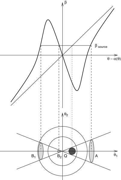
Fig. 3.54

Sketch of an axially symmetric lens. In the top panel, θ −α(θ) is plotted as a function of the angular separation θ from the center of the lens, together with the straight line β = θ. The three intersection points of the horizontal line at fixed β with the curve θ −α(θ) are the three solutions of the lens equation. The bottom image indicates the positions and sizes of the images on the observer’s sky. Here, Q is the unlensed source (which is not visible itself in the case of light deflection, of course!), and A, B1, B2 are the observed images of the source. The sizes of the images, and thus their fluxes, differ considerably; the inner image B2 is particularly weak in the case depicted here. The flux of B2 relative to that of image A depends strongly on the core radius of the lens; it can be so low as to render the third image unobservable. In the special case of a singular isothermal sphere, the innermost image is in fact absent. Adapted from P. Young et al. 1980, The double quasar Q0957 + 561 A,B—A gravitational lens image formed by a galaxy at z = 0.39, ApJ 241, 507, Fig. 6

3.11.2 Simple models

Axially symmetric mass distributions. The simplest models for gravitational lenses are those which are axially symmetric, for which $\varSigma ({\boldsymbol \xi }) =\varSigma (\xi )$ , where $\xi =\vert {\boldsymbol \xi }\vert$ denotes the distance of a point from the center of the lens in the lens plane. In this case, the deflection angle is directed radially inwards, and we obtain

$\displaystyle{ \hat{\alpha }= \frac{4GM(\xi )} {c^{2}\,\xi } = \frac{4G} {c^{2}\,\xi } \,2\pi \int _{0}^{\xi }\mathrm{d}\xi '\;\xi '\,\varSigma (\xi ')\;, }$

(3.69)

where M(ξ) is the mass within radius ξ. Accordingly, for the scaled deflection angle we have

$\displaystyle{ \alpha (\theta ) = \frac{m(\theta )} {\theta }:= \frac{1} {\theta } \,2\int _{0}^{\theta }\mathrm{d}\theta '\;\theta '\,\kappa (\theta ')\;, }$

(3.70)

where, in the last step, m(θ) was defined as the dimensionless mass within θ. Since ${\boldsymbol \alpha }$ and ${\boldsymbol \theta }$ are collinear, the lens equation becomes one-dimensional because only the radial coordinate needs to be considered,

$\displaystyle{ \beta =\theta -\alpha (\theta ) =\theta -\frac{m(\theta )} {\theta } \;. }$

(3.71)

An illustration of this one-dimensional lens mapping is shown in Fig. 3.54.

Example: Point-mass lens. For a point mass M, the dimensionless mass is independent of θ,

$\displaystyle{m(\theta ) = \frac{4GM} {c^{2}} \, \frac{D_{\mathrm{ds}}} {D_{\mathrm{d}}\,D_{\mathrm{s}}}\;,}$

reproducing the lens equation from Sect. 2.5.1 for a point-mass lens.

Example: Isothermal sphere. We saw in Sect. 2.4.2 that the rotation curve of our Milky Way is flat for large radii, and we know from Sect. 3.3.4 that the rotation curves of other spiral galaxies are flat as well. This indicates that the mass of a galaxy increases proportional to r, thus $\rho (r) \propto r^{-2}$ , or more precisely,

$\displaystyle{ \rho (r) = \frac{\sigma _{v}^{2}} {2\pi Gr^{2}}\;. }$

(3.72)

Here, σ _v is the one-dimensional velocity dispersion of stars in the potential of the mass distribution if the distribution of stellar orbits is isotropic. In principle, σ _v is therefore measurable spectroscopically from the line width. The mass distribution described by (3.72) is called a singular isothermal sphere (SIS). Because this mass model is of significant importance not only for the analysis of the lens effect, we will discuss its properties in a bit more detail.

The density (3.72) diverges for r → 0 as ρ ∝ r ⁻², so that the mass model cannot be applied up to the very center of a galaxy. However, the steep central increase of the rotation curve shows that the core region of the mass distribution, in which the density profile will deviate considerably from the r ⁻²-law, must be small for galaxies. Furthermore, the mass diverges for large r such that M(r) ∝ r. The mass profile thus has to be cut off at some radius in order to get a finite total mass. This cut-off radius is probably very large ( $\gtrsim 100\,\mathrm{kpc}$ for L ^∗-galaxies) because the rotation curves are flat to at least the outermost point at which they are observable.

/epubstore/S/P-Schneider/Extragalactic-Astronomy-And-Cosmology/OEBPS/A129044_2_En_3_Fig55_HTML.jpg

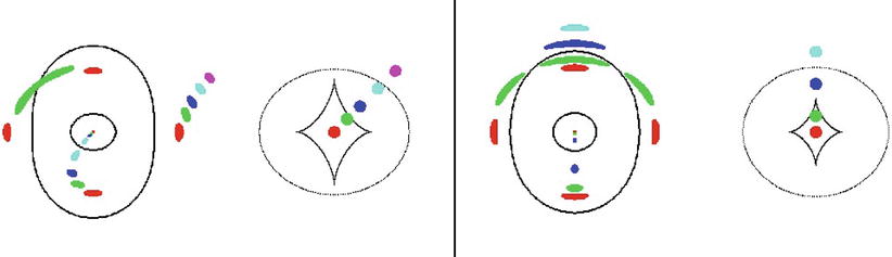
Fig. 3.55

Geometry of an ‘elliptical’ lens, whereby it is of little importance whether the surface mass density Σ is constant on ellipses (i.e., the mass distribution has elliptical isodensity contours) or whether an originally spherical mass distribution is distorted by an external tidal field. On the right-hand side in both panels, several different source positions in the source plane are displayed, each corresponding to a different color. The origin in the source plane is chosen as the intersection point of the line connecting the center of symmetry in the lens and the observer with the source plane (see also Fig. 2.31). Depending on the position of the source, 1, 3, or 5 images may appear in the lens plane (i.e., the observer’s sky); they are shown on the left-hand side of each panel. The curves in the lens plane are the critical curves, the location of all points for which μ → ∞. The curves in the source plane (i.e., on the right-hand side of each panel) are caustics, obtained by mapping the critical curves onto the source plane using the lens equation. Obviously, the number of images of a source depends on the source location relative to the location of the caustics. Strongly elongated images of a source occur close to the critical curves. Source: R. Narayan & M. Bartelmann 1996, Lectures on Gravitational Lensing, astro-ph/9606001

The SIS is an appropriate simple model for gravitational lenses over a wide range in radius since it seems to reproduce the basic properties of lens systems (such as image separation) quite well. The surface mass density is obtained from the projection of (3.72) along the line-of-sight,

$\displaystyle{ \varSigma (\xi ) = \frac{\sigma _{v}^{2}} {2G\xi }\;, }$

(3.73)

which yields the projected mass M(ξ) within radius ξ

$\displaystyle{ M(\xi ) = 2\pi \int _{0}^{\xi }\mathrm{d}\xi '\;\xi '\,\varSigma (\xi ') = \frac{\pi \sigma _{v}^{2}\xi } {G}\;. }$

(3.74)

With (3.69) the deflection angle can be obtained,

$\displaystyle\begin{array}{rcl} \hat{\alpha }(\xi )& =& 4\pi \left (\frac{\sigma _{v}} {c}\right )^{2},\quad \fbox{$\alpha (\theta ) = 4\pi \left (\frac{\sigma _{v}} {c}\right )^{2}\left (\frac{D_{\mathrm{ds}}} {D_{\mathrm{s}}} \right ) \equiv \theta _{\mathrm{E}}$}\;.{}\end{array}$

(3.75)

Thus the deflection angle for an SIS is constant and equals θ _E, and it depends quadratically on σ _v . θ _E is called the Einstein angle of the SIS. The characteristic scale of the Einstein angle is

$\displaystyle{ \theta _{\mathrm{E}} = 1.\!\!^{{\prime\prime}}15\left ( \frac{\sigma _{v}} {200\,\mathrm{km/s}}\right )^{2}\left (\frac{D_{\mathrm{ds}}} {D_{\mathrm{s}}} \right )\;, }$

(3.76)

from which we conclude that the angular scale of the lens effect in galaxies is about an arcsecond for massive galaxies. The lens equation (3.71) for an SIS is

$\displaystyle{ \beta =\theta -\theta _{\mathrm{E}}\;\frac{\theta } {\left \vert \theta \right \vert }\;, }$

(3.77)

where we took into account the fact that the deflection angle is negative for θ < 0 since it is always directed inwards.

Solution of the lens equation for the singular isothermal sphere. If $\left \vert \beta \right \vert <\theta _{\mathrm{E}}$ , two solutions of the lens equation exist,

$\displaystyle{ \theta _{1} =\beta +\theta _{\mathrm{E}}\quad,\quad \theta _{2} =\beta -\theta _{\mathrm{E}}\;. }$

(3.78)

Without loss of generality, we assume β ≥ 0; then $\theta _{1} >\theta _{\mathrm{E}} > 0$ and $0 >\theta _{2} > -\theta _{\mathrm{E}}$ : one image of the source is located on either side of the lens center, and the separation of the images is

$\displaystyle\begin{array}{rcl} & & \fbox{$\varDelta \theta =\theta _{1} -\theta _{2} = 2\theta _{\mathrm{E}} = 2.\!\!^{{\prime\prime}}3\left ( \frac{\sigma _{v}} {200\,\mathrm{km/s}}\right )^{2}\left (\frac{D_{\mathrm{ds}}} {D_{\mathrm{s}}} \right )$}\;.{}\end{array}$

(3.79)

Thus, the angular separation of the images does not depend on the position of the source. For massive galaxies acting as lenses it is of the order of somewhat more than 1 arcsec. For $\beta >\theta _{\mathrm{E}}$ only one image of the source exists, at θ ₁, meaning that it is located on the same side of the center of the lens as the unlensed source.

For the magnification, we find

$\displaystyle{ \mu (\theta ) = \frac{\left \vert \theta /\theta _{\mathrm{E}}\right \vert } {\left \vert \left \vert \theta /\theta _{\mathrm{E}}\right \vert - 1\right \vert }\;. }$

(3.80)

If $\theta \approx \theta _{\mathrm{E}}$ , μ is very large. Such solutions of the lens equation exist for $\left \vert \beta \right \vert \ll \theta _{\mathrm{E}}$ , so that sources close to the center of the source plane may be highly magnified. If β = 0, the image of the source will be a ring of radius θ = θ _E, a so-called Einstein ring .

More realistic models. Mass distributions occurring in nature are not expected to be truly symmetric. The ellipticity of the mass distribution or external shear forces (caused, for example, by the tidal gravitational field of neighboring galaxies) will disturb the symmetry. The lensing properties of the galaxy will change by this symmetry breaking. For example, more than two images may be generated. Figure 3.55 illustrates the lens properties of such elliptical mass distributions. One can see, for example, that pairs of images, which are both heavily magnified, may be observed with a separation significantly smaller than the Einstein radius of the lens. Nevertheless, the characteristic image separation is still of the order of magnitude given by (3.79).

3.11.3 Examples for gravitational lenses

Currently, about 200 gravitational lens systems are known in which a galaxy acts as the lens. Many of them were discovered serendipitously, but most were found in systematic searches for lens systems. Amongst the most important lens surveys are: (1) The Cosmic Lens All-Sky Survey (CLASS). About 15 000 radio sources with a flat radio spectrum (these often contain compact radio components, see Sect. 5.1.3) were scanned for multiple components, using the VLA. Possible multiple image candidate were then studied in more detail. From this survey, 22 lens systems were found. These numbers immediately show that strong lensing is a rather rare phenomenon, with roughly 1 out of 1000 distant sources being lensed by a foreground galaxy. (2) The SDSS Quasar Lens Search (SQLS). The multicolor image data from SDSS were used to study images of quasars from the spectroscopic SDSS survey, to search for indications of multiple images. In this survey, 28 lens systems were found. Due to the resolution of the SDSS imaging data, this survey preferentially selected lenses with large image separations. (3) The Sloan Lens Advanced Camera for Surveys (SLACS). If a galaxy lies directly behind a closer galaxy, then the resulting spectrum will be a superposition of the spectra of the two galaxies. In SLACS, the galaxy spectra of the SDSS were searched for indications of the presence of two different redshifts. Candidate systems were then imaged with the HST, to find evidence for multiple images or (partial) Einstein rings. The SLACS survey yielded 85 strong lensing systems.

The different search strategies for lenses all have their merits. For example, radio lenses, as found by CLASS, can often be studied with much higher angular resolution, due to the availability of Very Long Baseline Interferometry (VLBI). However, many of these radio sources are very faint in the optical, and determining their redshift from optical spectroscopy can be highly challenging. Indeed, the source redshift is known only for half of the CLASS lenses. This problem is absent in the SLACS survey, since the redshifts of both (foreground and background) galaxies were determined at the stage were candidate systems were identified. Furthermore, the redshift distribution of the lenses and sources are quite different; of the three surveys mentioned, SLACS has the lowest lens and source redshifts, due to the limiting magnitude of the spectroscopic galaxy survey.

Most lens galaxies are ellipticals; in fact, spirals occur in only ∼ 10 % of all lens systems. The reason for that can be traced back to the fact the massive ellipticals are more abundant than spirals, as can be seen in the right-hand panel of Fig. 3.52. Since the mass does not only determine the image separation that a lens can generate, but also the effective area of the sky in which a background source must be located in order to be multiply imaged, it turns out that ellipticals dominate the lensing probability distribution.¹³

QSO 0957+561, the first double quasar. The first lens system was discovered in 1979 by Walsh, Carswell & Weymann when the optical identification of a radio source showed two point-like optical sources (see Fig. 3.56). Both could be identified as quasars located at the same redshift of z _s = 1. 41 and having very similar spectra (see Fig. 3.57). Deep optical images of the field show an elliptical galaxy situated between the two quasar images, at a redshift of z _d = 0. 36. The galaxy is so massive and so close to image B of the source that it has to produce a lens effect. However, the observed image separation of $\varDelta \theta = 6.\!\!^{{\prime\prime}}1$ is considerably larger than expected from the lens effect by a single galaxy (3.79). The explanation for this is that the lens galaxy is located in a cluster of galaxies; the additional lens effect of the cluster adds to that of the galaxy, boosting the image separation to a large value. The lens system QSO 0957+561 was observed in all wavelength ranges, from the radio to the X-ray. The two images of the quasar are very similar at all λ, including the VLBI structure (Fig. 3.57)—as would be expected since the lens effect is independent of the wavelength, i.e., achromatic.

/epubstore/S/P-Schneider/Extragalactic-Astronomy-And-Cosmology/OEBPS/A129044_2_En_3_Fig56_HTML.jpg

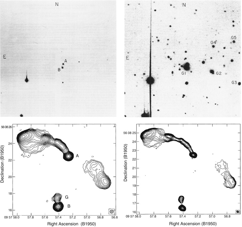
Fig. 3.56

Top: optical images of the double quasar QSO 0957+561. The image on the top left has a short exposure time; here, the two point-like images A & B of the quasar are clearly visible. In contrast, the image on the top right has a longer exposure time, showing the lens galaxy G1 between the two quasar images. Several other galaxies (G2–G5) are visible as well. The lens galaxy is a member of a cluster of galaxies at z _d = 0. 36. Bottom: two radio maps of QSO 0957+561, observed with the VLA at 6 cm (left) and 3.6 cm (right), respectively. The two images of the quasar are denoted by A & B; G is the radio emission of the lens galaxy. The quasar has a radio jet, which is a common property of many quasars (see Sect. 5.1.3). On small angular scales, the jet can be observed by VLBI techniques in both images (see Fig. 3.57). On large scales only a single image of the jet exists, seen in image A; this property should be compared with Fig. 3.55 where it was demonstrated that the number of images of a source (component) depends on its position in the source plane. Source: Top: P. Young et al. 1980, The double quasar Q0957 + 561 A,B—A gravitational lens image formed by a galaxy at z = 0.39, ApJ 241, 507, p. 508, 509, Fig. 1a,b. ©AAS. Reproduced with permission. Bottom: M. Harvanek et al. 1997, High Dynamic Range VLA Observations of the Gravitationally Lensed Quasar 0957+561, AJ 114, 2240, p. 2242, Fig. 1. ©AAS. Reproduced with permission

QSO PG1115+080. In 1980, the so-called triple quasar was discovered, composed of three optical quasars at a maximum angular separation of just below 3″. Component A is significantly brighter than the other two images (B, C; see Fig. 3.58, left). In high-resolution images it was found that the brightest image is in fact a double image: A is split into A1 and A2. The angular separation of the two roughly equally bright images is $\sim 0.\!\!^{{\prime\prime}}5$ , which is considerably smaller than all other angular separations in this system. The four quasar images have a redshift of z _s = 1. 72, and the lens is located at z _d = 0. 31. The image configuration is one of those that are expected for an elliptical lens, see Fig. 3.55.

With the NIR camera NICMOS on-board HST, not only the quasar images and the lens galaxy were observed, but also a nearly complete Einstein ring (Fig. 3.58, right). The source of this ring is the host galaxy of the quasar (see Sect. 5.4.5) which is substantially redder than the active galactic nucleus itself.

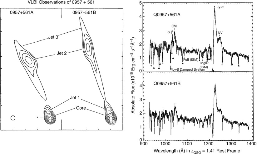
/epubstore/S/P-Schneider/Extragalactic-Astronomy-And-Cosmology/OEBPS/A129044_2_En_3_Fig57_HTML.jpg

Fig. 3.57

Left: milliarcsecond structure of the two images of the quasar QSO 0957+561, a VLBI map at 13 cm wavelength. Both quasar images show a core-jet structure, and it is clearly seen that they are mirror-symmetric, as predicted by lens models. Right: spectra of the two quasar images QSO 0957+561A,B, observed by the Faint Object Camera (FOC) on-board HST. The similarity of the spectra, in particular the identical redshift, is a clear indicator of a common source of the two quasar images. The broad Lyα-line, in the wings of which an Nv-line is visible, is virtually always the strongest emission line in quasars. Source: Left: M. Gorenstein et al. 1988, VLBI observations of the gravitational lens system 0957+561—Structure and relative magnification of the A and B images, ApJ 334, 42, p. 53, Fig. 5. ©AAS. Reproduced with permission. Right: A.G. Michalitsianos et al. 1997, Ly alpha Absorption-Line Systems in the Gravitational Lens Q0957+561, ApJ 474, 598, p. 599, Fig. 1. ©AAS. Reproduced with permission

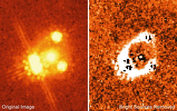
/epubstore/S/P-Schneider/Extragalactic-Astronomy-And-Cosmology/OEBPS/A129044_2_En_3_Fig58_HTML.jpg

Fig. 3.58

A NIR image of QSO 1115+080 is shown on the left, as observed with the NICMOS camera on-board HST. The double structure of image A (the left of the QSO images) is clearly visible, although the image separation of the two A components is less than 0. ^{′ ′} 5. The lens galaxy, located in the ‘middle’ of the QSO images, has a much redder spectral energy distribution than the quasar images. In the right-hand panel, the quasar images and the lens galaxy have been subtracted. What remains is a nearly closed ring; the light of the galaxy which hosts the active galactic nucleus is imaged into an Einstein ring. Credit: C. Impey (University of Arizona) & NASA

From the image configuration in such a quadruple system, the mass of the lens within the images can be estimated very accurately. The four images of the lens system trace a circle around the center of the lens galaxy, the radius of which can be identified with the Einstein radius of the lens. From this, the mass of the lens within the Einstein radius follows immediately because the Einstein radius is obtained from the lens equation (3.71) by setting β = 0. Therefore, the Einstein radius is the solution of the equation

$\displaystyle{\theta =\alpha (\theta ) = \frac{m(\theta )} {\theta } \;,}$

$\displaystyle{m(\theta _{\mathrm{E}}) = \frac{4GM(\theta _{E})} {c^{2}} \, \frac{D_{\mathrm{ds}}} {D_{\mathrm{d}}\,D_{\mathrm{s}}} =\theta _{ \mathrm{E}}^{2}\;.}$

/epubstore/S/P-Schneider/Extragalactic-Astronomy-And-Cosmology/OEBPS/A129044_2_En_3_Fig59_HTML.jpg

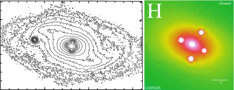
Fig. 3.59

Left: in the center of a nearby spiral galaxy, four point-like sources were found whose spectra show strong emission lines. This image from the CFHT clearly shows the bar structure in the core of the lens galaxy. An HST/NICMOS image of the center of QSO 2237+0305 is shown on the right. The central source is not a fifth quasar image but rather the bright nucleus of the lens galaxy. Credit: Left: H.K.C. Yee 1988, High-resolution imaging of the gravitational lens system candidate 2237+030, AJ 95, 1331, p. 1332, Fig. 4. ©AAS. Reproduced with permission. Right: CASTLES-Collaboration, C.S. Kochanek

This equation is best written as

$\displaystyle{ \fbox{$M(\theta _{\mathrm{E}}) =\pi \left (D_{\mathrm{d}}\theta _{\mathrm{E}}\right )^{2}\varSigma _{ \mathrm{cr}}$}\;, }$

(3.81)

which is readily interpreted:

The mass within θ _E of a lens follows from the fact that the mean surface mass density within θ _E equals the critical surface mass density Σ _cr. A more accurate determination of lens masses is possible by means of detailed lens models. For quadruple image systems, the masses can be derived with a precision of a few percent—these are the most precise mass determinations in (extragalactic) astronomy.

QSO 2237+0305: The Einstein Cross. A spectroscopic survey of galaxies found several unusual emission lines in the nucleus of a nearby spiral galaxy which cannot originate from the galaxy itself. Instead, they are emitted by a background quasar at redshift z _s = 1. 7 situated exactly behind this spiral. High-resolution images show four point sources situated around the nucleus of this galaxy, with an image separation of $\varDelta \theta \approx 1.\!\!^{{\prime\prime}}8$ (Fig. 3.59). The spectroscopic analysis of these point sources revealed that all four are images of the same quasar (Fig. 3.60).

/epubstore/S/P-Schneider/Extragalactic-Astronomy-And-Cosmology/OEBPS/A129044_2_En_3_Fig60_HTML.jpg

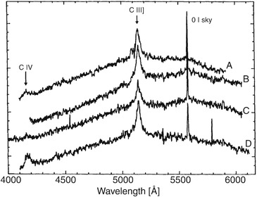
Fig. 3.60

Spectra of the four images of the quasar 2237+0305, observed with the CFHT. As is clearly visible, the spectral properties of these four images are very similar; this is the final proof that we are dealing with a lens system here. Measuring the individual spectra of these four very closely spaced sources is extremely difficult and can only be performed under optimum observing conditions. Source: G. Adam et al. 1989, Observations of the Einstein Cross 2237+030 with the TIGER Integral Field Spectrograph, A&A 208, L15, p. L17, Fig. 6. ©ESO. Reproduced with permission

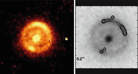
/epubstore/S/P-Schneider/Extragalactic-Astronomy-And-Cosmology/OEBPS/A129044_2_En_3_Fig61_HTML.jpg

Fig. 3.61

The radio source B1938+666 with z _s = 2. 059 is seen to be multiply imaged (contours in the right-hand part); here, the radio source consists of two components, one of which is imaged fourfold, the other twofold. A NIR image taken with the NICMOS camera on-board the HST (left-hand part, also shown on the right in gray-scale) shows the lens galaxy (z _d = 0. 88) in the center of an Einstein ring that originates from the stellar light of the host galaxy of the active galactic nucleus. Credit: L.J. King, based on data from King et al. 1998, A complete infrared Einstein ring in the gravitational lens system B1938+666, MNRAS 295, L41

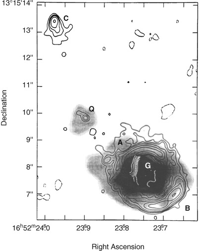
/epubstore/S/P-Schneider/Extragalactic-Astronomy-And-Cosmology/OEBPS/A129044_2_En_3_Fig62_HTML.jpg

Fig. 3.62

The quasar MG 1654+13 shows, in addition to the compact radio core (Q), two radio lobes; the northern lobe is denoted by C, whereas the southern lobe is imaged into a ring. An optical image is displayed in gray-scales, showing not only the quasar at Q (z _s = 1. 72) but also a massive foreground galaxy (G) at z _d = 0. 25 that is responsible for the lensing of the lobe into an Einstein ring. The mass of this galaxy within the ring can be derived with a precision of ∼ 1 %. Credit: G. Langston, based on data from Langston et al. 1989, MG 1654+1346 - an Einstein Ring image of a quasar radio lobe, AJ 97, 1283

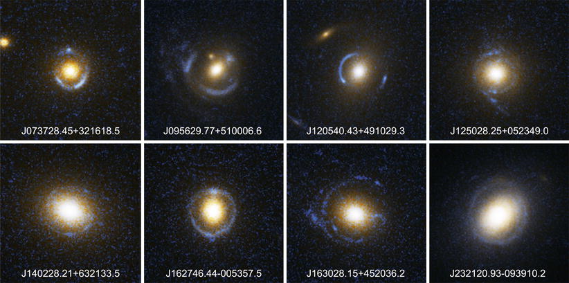
/epubstore/S/P-Schneider/Extragalactic-Astronomy-And-Cosmology/OEBPS/A129044_2_En_3_Fig63_HTML.jpg

Fig. 3.63

Eight strong lens systems from the SLACS survey. In contrast to multiply imaged quasars, the images of the lensed source are extended, and often highly elongated or even mapped onto a full Einstein ring. Such extended images can probe the gravitational potential of the lens at far more locations than a few point-like images, and thus potentially provide more information about the mass distribution. Credit: NASA, ESA, and the SLACS Survey team: A. Bolton (Harvard/ Smithsonian), S. Burles (MIT), L. Koopmans (Kapteyn), T. Treu (UCSB), and L. Moustakas (JPL/Caltech)

The images in this system are positioned nearly symmetrically around the lens center; this is also a typical lens configuration which may be caused by an elliptical lens (see Fig. 3.55). The Einstein radius of this lens is $\theta _{\mathrm{E}} \approx 0.\!\!^{{\prime\prime}}9$ , and we can determine the mass within this radius with a precision of ∼ 3 %.

Einstein rings. More examples of Einstein rings are displayed in Figs. 3.61 and 3.62. The first of these is a radio galaxy, with its two radio components being multiply imaged by a lens galaxy—one of the two radio sources is imaged into four components, the other mapped into a double image. In the NIR the radio galaxy is visible as a complete Einstein ring. This example shows very clearly that the appearance of the images of a source depends on the source size: to obtain an Einstein ring a sufficiently extended source is needed.

At radio wavelengths, the quasar MG 1654+13 consists of a compact central source and two radio lobes. As we will discuss in Sect. 5.1.3, this is a very typical radio morphology for quasars. One of the two lobes has a ring-shaped structure, which prior to this observation had never been observed before. An optical image of the field shows the optical quasar at the position of the compact radio component and, in addition, a bright elliptical galaxy right in the center of the ring-shaped radio lobe. This galaxy has a significantly lower redshift than the quasar and hence is the gravitational lens responsible for imaging the lobe into an Einstein ring. The SLACS survey has found a large number of Einstein rings, as shown in Fig. 3.63.

3.11.4 Applications of the lens effect

Mass determination. As mentioned previously, the mass within a system of multiple images can be determined directly, sometimes very precisely. Even without a specific model, an estimate of the Einstein radius from the location of the multiple images immediately yields a mass estimate from (3.81). Its accuracy depends on the detailed image configuration but can be substantially better than 10 % for quadruple image systems. Once the mass distribution is quantitatively modeled, such as it reproduces the observed image positions, the mass within the Einstein radius can be determined with very high accuracy.

Since the length scale in the lens plane (at given angular scale) and Σ _cr depend on H ₀, these mass estimates scale with H ₀. For instance, for QSO 2237+0305, a mass within $0.\!\!^{{\prime\prime}}9$ of $(1.08 \pm 0.02)h^{-1} \times 10^{10}M_{\odot }$ is derived. An even more precise determination of the mass was obtained for the lens galaxy of the Einstein ring in the system MG 1654+13 (Fig. 3.62). The dependence on the other cosmological parameters is comparatively weak, especially at low redshifts of the source and the lens. Most lens galaxies are early-type galaxies (ellipticals); from the determination of their mass it is concluded that ellipticals contain dark matter, as spirals do. For example, the fraction of dark matter inside the Einstein ring 1938+666 (Fig. 3.61) is 0.20 if a Salpeter initial mass function is assumed, but increases to 0.55 if a (more realistic) IMF is used which flattens for masses below ∼ 1M _⊙.

Similar results have been obtained for large number of lens galaxies. In the lens system 1933+503, a three-component radio source is lensed into a total of ten images by a spiral lens galaxy, where two of the radio components have four images, the third one has two. Using the observed rotation curve of the spiral, a clear decomposition of the baryonic matter (located in a disk) and the dark matter (distributed in an extended halo) became feasible. The dark matter fraction projected inside the effective radius in this lens galaxy is about 40 % for a realistic initial mass function. Comparing the light distribution of the lens, and translating this into a stellar mass, using stellar population synthesis, it is found that a bottom-heavy IMF (like Salpeter) is strongly disfavored compared to those with a flattening at low masses, and analogous results were found for other spiral lens galaxies as well. At least for one early-type lens galaxy, a bottom-heavy IMF like the Salpeter function is actually ruled out, as otherwise the stellar mass would exceed the lensing mass.

Mass profile and dark matter fraction. Whereas one can determine the mass within the Einstein radius with high accuracy, in a typical lens configuration one cannot say much about the density profile. There are special lens systems where this becomes possible, namely those where the images span a large range in separation from the lens center. But even in those systems, conclusions about the slope of the profile are not necessarily very robust. An exception to this occurs for lens systems where two sources at different redshift are lensed by the same galaxy; in this case, one has two Einstein radii (one corresponding to each source redshift), and one can determine the masses at two different radii.

However, if it is possible to combine the mass estimate within the Einstein radius with a different mass estimate at a different radius, we can obtain information about the density profile. Another mass estimate is obtained from the stellar kinematics in the (early-type) lens galaxies, studied via spectroscopy. The velocity dispersion of stars, which determines the absorption line width, depends on the local gravitational potential via the virial theorem, and is typically estimated at the effective radius. Thus, if the effective radius is significantly different from the Einstein radius, which is the case in most lens systems, the slope of the mass profile can be estimated. It turns out that the isothermal profile, ρ ∝ r ⁻², is a very good description for most lens galaxies, with only small variations of the slope being observed.

This is a very surprising result! To see why, let us recall that the brightness profile of ellipticals is approximated by a de Vaucouleurs profile, which differs substantially from a projected isothermal profile. Thus, the first conclusion from this is that the mass profile does not follow the light profile; hence, beside the stars, there must be an additional mass component in these galaxies. From the spectral energy distribution of the stellar population in the lens galaxies, one can estimate the mass-to-light ratio of the stellar population, hence the stellar mass within the Einstein radius. Comparing with the mass determined from lensing, one finds that about half the mass within the Einstein radius is stellar; the other half is dark matter. In agreement with what was said before, the fraction of dark matter inside the Einstein radius varies between ∼ 30 and ∼ 70 %, with more massive lenses having a higher dark matter fraction. As we will see in Sect. 7.6.1, the mass profile of the dark matter is predicted to differ substantially from an isothermal profile, at least at small scales. However, the results about the mass profile tell us that the distributions of stars and of dark matter conspire in such a way that the sum of them is approximately isothermal. Needless to say that this results is an important constraint for the theory of galaxy formation and evolution.

Mass fundamental plane. One finds from the large sample of SLACS lenses that the mass-to-light ratio of lens galaxies increases with mass, in concordance with what was discussed in relation with the fundamental plane (Sect. 3.4.3). In fact, lensing accurately measures the mean surface mass density within the Einstein radius—see (3.81). For the SLACS lenses, the typical Einstein radius is about 0. 6R _e. Together with the fact that the slope of the mass profile is isothermal with good accuracy, the mean surface mass density within half the effective radius can be determined. This allows us to write a ‘fundamental plane’-relation in terms of the surface mass density, instead of the surface brightness. From the virial theorem, one would conclude

$\displaystyle{\sigma _{0}^{2} \propto M/R \propto \varSigma _{\mathrm{ e2}}\,R_{\mathrm{e}}\;,}$

where we specialized $R = R_{\mathrm{e}}/2$ , and Σ _e2 is the mean surface mass density within half the effective radius. In other words, this implies a relation of the form

$\displaystyle{ R_{\mathrm{e}} \propto \sigma _{0}^{a}\,\varSigma _{ \mathrm{e2}}^{b}\;, }$

(3.82)

with a = 2 and $$b = -1$$

. Indeed, the SLACS lenses define such a mass-based fundamental plane, with a ≈ 2 and b ≈ −1, and their dispersion about this mass-based fundamental plane is even slightly smaller than that around the standard fundamental plane (3.30), based on luminosity. This shows that the tilt of the fundamental plane is indeed due to a varying mass-to-light ratio as a function of galaxy mass, as described by (3.32).

Shape of the mass distribution. From modeling gravitational lens systems, the ellipticity of the mass distribution and the orientation of the major axis can be determined.¹⁴ It is interesting to study whether ellipticity and orientation of the mass agree with that of the light distribution. Indeed, this is the case: The orientation of the mass distribution agrees with that of the light distribution, with a dispersion of the difference between the two position angles of ∼ 10^∘. The same holds for the ellipticity, or axis ratio; in early-type lens galaxies, the axis ratios of mass and light agree to within 10 %.

These are no trivial statements, given that about half the mass inside the Einstein radius is dark. The shape of the dark matter distribution must be quite similar to, but not identical as that of the stars. Thus, whereas the radial density profile of dark matter and stars are quite different, their shapes are similar.

Environmental effects. Detailed lens models show that the light deflection of most gravitational lenses is affected by an external tidal field. This is due to the fact that lens galaxies are often members of galaxy groups which contribute to the light deflection as well. In some cases the members of the group were identified. Mass properties of the corresponding group can be derived from the strength of this external influence.

Determination of the Hubble constant. The light travel times along the different paths (according to the multiple images) are not the same. On the one hand the paths have different geometrical lengths, and on the other hand the light rays traverse different depths of the gravitational potential of the lens, resulting in a (general relativistic) time dilation effect. The difference in the light travel times Δ t is measurable because luminosity variations of the source are observed at different times in the individual images. Δ t can be measured from this difference in arrival time, called the time delay.

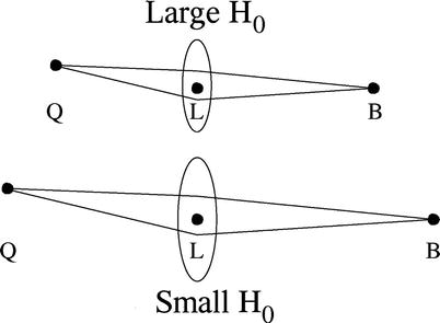
/epubstore/S/P-Schneider/Extragalactic-Astronomy-And-Cosmology/OEBPS/A129044_2_En_3_Fig64_HTML.jpg

Fig. 3.64

Lens geometry in two universes with different Hubble constant. All observables are dimensionless—angular separations, flux ratios, redshifts—except for the difference in the light travel time. This is larger in the universe at the bottom than in the one at the top; hence, $\varDelta t \propto H_{0}^{-1}$ . If the time delay Δ t can be measured, and if one has a good model for the mass distribution of the lens, then the Hubble constant can be derived from measuring Δ t. Source: R. Narayan & M. Bartelmann 1996, Lectures on Gravitational Lensing, astro-ph/9606001

It is easy to see that Δ t depends on the Hubble constant, or in other words, on the size of the Universe. If a universe is twice the size of our own, Δ t would be twice as large as well—see Fig. 3.64. Thus if the mass distribution of the lens can be modeled sufficiently well, by modeling the geometry of the image configuration, then the Hubble constant can be derived from measuring the difference in the light travel time. To date, Δ t has been measured in about 20 lens systems (see Fig. 3.65 for an example). Based on ‘plausible’ lens models we can derive values for the Hubble constant. Early results obtained with that method often yielded rather small values of H ₀, probably because of employing too simple mass models for the lens. The main difficulty here is that the mass distribution in lens galaxies cannot unambiguously be derived from the positions of the multiple images.

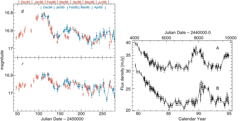
/epubstore/S/P-Schneider/Extragalactic-Astronomy-And-Cosmology/OEBPS/A129044_2_En_3_Fig65_HTML.jpg

Fig. 3.65

Left: optical light curves of the double quasar 0957+561 in two broad-band filters. The light curve of image A is displayed in red and that of image B in blue, where the latter is shifted in time by 417 days. With this shift, the two light curves are made to coincide—this light travel time difference of 417 days is determined with an accuracy of ∼ ±3 days. Right: radio light curves of QSO 0957+561A,B at 6 cm. From these radio measurements Δ t can also be measured, and the corresponding value is compatible with that obtained from optical data. Source: Left: T. Kundić et al. 1997, A Robust Determination of the Time Delay in 0957+561A, B and a Measurement of the Global Value of Hubble’s Constant, ApJ 482, 75, p. 79, Fig. 3. ©AAS. Reproduced with permission. Right: D.B. Haarsma et al. 1997, The 6 Centimeter Light Curves of B0957+561, 1979–1994: New Features and Implications for the Time Delay, ApJ 479, 102, p. 104, Fig. 1. ©AAS. Reproduced with permission

However, much more detailed models are feasible for lens systems where an extended source component is lensed, e.g., into an Einstein ring, in addition to multiple images of a compact component. Recently, results from two such detailed modeling efforts became available, resulting in H ₀ ≈ 71 and $79\,\mathrm{km}\,\mathrm{s}^{-1}\mathrm{Mpc}^{-1}$ , respectively, with an estimated error of about 5 %. These measurements are in good agreement with those from the distance ladder—see (3.50). We should note, however, that the determination of H ₀ from time delay lenses is affected by the so-called mass-sheet degeneracy (see Problem 3.5), which may lead to an increased error budget. In Sect. 6.4.4 we will discuss the value of H ₀ determinations from lens time delays in a slightly different context.

The ISM in lens galaxies. Since the same source is seen along different sight lines passing through the lens galaxy, the comparison of the colors and spectra of the individual images provides information on reddening and on dust extinction in the ISM of the lens galaxy. From such investigations it was shown that the extinction in ellipticals is in fact very low, as is to be expected from the small amount of interstellar medium they contain, whereas the extinction is considerably higher for spirals. These analyses also enable us to study the relation between extinction and reddening, and from this to search for deviations from the Galactic reddening law (2.21)—see Fig. 2.7. In fact, the constant of proportionality R _V is different in other galaxies, indicating a different composition of the dust, e.g., with respect to the chemical composition and to the size distribution of the dust grains.

3.12 Problems

3.1. Central surface brightness of disk galaxies. Assume the validity of Freeman’s law, and consider a spiral galaxy with central surface brightness $\mu _{0} = 21.5\,\mathrm{mag/arcsec^{2}}$ at the distance of the Virgo cluster, i.e., D = 16 Mpc.

With the absolute magnitude of the Sun in the B-band of M _⊙, B = 5. 54, calculate the central surface brightness of the galaxy in Solar luminosities per pc².

The disk is seen to have an exponential surface brightness, with angular scale length of θ _R = 50″. What is the total luminosity of the disk?

3.2. Properties of the Salpeter IMF. Let us assume that the stellar mass function has the same shape as the Salpeter IMF (3.36), with m _L = 0. 1M _⊙ and m _U = 70M _⊙. We define m _m50 such that half of the stellar mass is contained in stars with mass below m _m50, the other half in stars with m > m _m50. Similarly, we define m _L50 such that half of the luminosity from the stellar population is due to stars with m < m _L50. Calculate the masses m _m50 and m _L50, the latter by assuming that the luminosity of stars scales with mass as $L \propto m^{3}$ . From a comparison of m _m50 and m _L50, draw conclusions about the relative importance of low- and high-mass stars for the mass budget and the luminosity of the stellar population.

3.3. Observable supernova rate. The rate of Type Ia supernovae explosions is about $3 \times 10^{-5}\,\mathrm{Mpc^{-3}\,yr^{-1}}$ . Assume that a photometric supernova survey is carried out with a sensitivity which allows the detection of these sources out to a distance of 500 Mpc. How many square degrees of the sky need to be surveyed in order to find 10 SNe Ia per year?

3.4. Obtaining the luminosity function of galaxies. A galaxy survey is carried out over a solid angle ω, and only objects with distance ≤ D _lim shall be considered. The galaxy survey is flux-limited, which means that only sources with flux above a threshold, S ≥ S _min, can be observed.

Show that the total volume in which galaxies are considered for the survey is $V _{\mathrm{tot}} = D_{\mathrm{lim}}^{3}\,\omega /3$ .

Calculate the volume V _max(L) within which we can observe galaxies with luminosity L.

Let N(L) be the number of galaxies found with luminosity smaller than L. Show that the luminosity function is then determined as

$\displaystyle{ \varPhi (L) = \frac{1} {V _{\mathrm{max}}(L)}\,\frac{\mathrm{d}N(L)} {\mathrm{d}L} \;. }$

(3.83)

3.5. Mass-sheet degeneracy. For a given gravitational lens system, suppose you have a perfect model: a surface mass density profile $\kappa ({\boldsymbol \theta })$ such that the corresponding scaled deflection angle ${\boldsymbol \alpha }({\boldsymbol \theta })$ , inserted into the lens equation (3.64), yields a solution for all image positions ${\boldsymbol \theta }_{i}$ , i.e., there exist a source position ${\boldsymbol \beta }$ such that ${\boldsymbol \beta }={\boldsymbol \theta } _{i} -{\boldsymbol \alpha } ({\boldsymbol \theta }_{i})$ for all images i.

Consider now a family of lens models, described by the surface mass density

$\displaystyle{ \kappa _{\lambda }({\boldsymbol \theta }) = (1-\lambda ) +\lambda \kappa ({\boldsymbol \theta })\;. }$

(3.84)

Thus, $\kappa _{\lambda }({\boldsymbol \theta })$ is obtained by scaling the original mass distribution by a factor λ, and adding a constant surface mass density of amplitude (1 −λ). Calculate the scaled deflection angle ${\boldsymbol \alpha }_{\lambda }({\boldsymbol \theta })$ corresponding to the surface mass density κ _λ .

Derive the lens equation corresponding to the new surface mass density (3.84) and show that there exists a source position ${\boldsymbol \beta }_{\lambda } ={\boldsymbol \beta } /\lambda$ such that the image positions ${\boldsymbol \theta }_{i}$ all satisfy the new lens equation. Hence, the new mass distribution κ _λ describes the image position equally well as the original distribution κ, for all λ ≠ 0. This implies that from image positions alone, one can not distinguish between κ and κ _λ .

Calculate the magnification $\mu _{\lambda }({\boldsymbol \theta })$ for the new mass distribution in terms of the magnification $\mu ({\boldsymbol \theta })$ of the original mass distribution. Show that one cannot distinguish between these mass distributions from considering the flux ratios (which is the same as the magnification ratios) of the images.

Footnotes

Isophotes are contours along which the surface brightness of a source is constant. If the light profile of a galaxy is elliptical, then its isophotes are ellipses.

The morphological classification recently had a revival, with the Galaxy Zoo project. Its goal was to obtain the morphological classification of millions of galaxies from the Sloan Digital Sky Survey (SDSS), carried out by the general public—i.e., everyone interested could participate. Every galaxy was seen and classified by many different participants, so that misclassifications of individuals get corrected ‘democratically’. In its first year of existence, more than 150 000 people participated, yielding the classification of ∼ 50 × 10⁶ galaxies. A large number of publications are based on the results of the Galaxy Zoo project.

If a ≥ b ≥ c denote the lengths of the major axes of an ellipsoid, then it is called an oblate spheroid ( = rotational ellipsoid) if a = b > c, whereas a prolate spheroid is specified by a > b = c. If all three axes are different, it is called triaxial ellipsoid.

Note that in a gas like air, scattering between molecules occurs frequently, which drives the velocity distribution of the molecules towards an isotropic Maxwellian, i.e., the thermal distribution.

This consideration is strongly simplified insofar as the given relations are only valid in this form for spherical mass distributions. The rotational velocity produced by an oblate (disk-shaped) mass distribution is more complicated to calculate; for instance, for an exponential mass distribution in a disk, the maximum of v _lum occurs at ∼ 2. 2h _R , with a Kepler decrease, $v_{\mathrm{lum}} \propto R^{-1/2}$ , at larger radii.

We point out explicitly once more that the surface brightness does not depend on the distance of a source.

The SDSS spectroscopic sample is flux limited, i.e., it contains (almost) all galaxies in its sky region with a flux S > S _lim. If we restrict the sample to a maximum distance D _max, then the sample is also complete for luminosities $L > 4\pi S_{\mathrm{lim}}D_{\mathrm{max}}^{2}$ .

In red giants, nuclear burning of hydrogen occurs in a shell around the core which is formed by helium-rich gas. As shell burning proceeds, the helium core becomes more massive, as well as hotter, and the stellar luminosity increases. Once a certain threshold in the core temperature is reached, the central helium core ignites, and the stars quickly evolved to the horizontal branch. The threshold core temperature then corresponds to the maximum luminosity of a red giant.

To calibrate the luminosity of SN Ia, the surveys for determining Cepheid distances were preferentially targeted towards those galaxies in which a SN Ia had been observed.

Recall that the surface brightness does not depend on distance, as long as we are considering objects in the nearby Universe, i.e., with redshifts z ≪ 1.

Here, Γ(x) is the Gamma function, defined by

$\displaystyle{ \varGamma (x) =\int _{ 0}^{\infty }\mathrm{d}y\;y^{(x-1)}\,\mathrm{e}^{-y}\;. }$

(3.57)

For positive integers, $\varGamma (n + 1) = n!$ . We have $\varGamma (0.7) \approx 1.30$ , Γ(1) = 1, $\varGamma (1.3) \approx 0.90$ . Since these values are all close to unity, $l_{\mathrm{tot}} \sim \varPhi ^{{\ast}}L^{{\ast}}$ is a good approximation for the luminosity density.

To characterize the strength of a gravitational field, we refer to the gravitational potential Φ. The ratio Φ∕c ² is dimensionless and therefore well suited to distinguishing between strong and weak gravitational fields. For weak fields, $\vert \varPhi \vert /c^{2} \ll 1$ . Another possible way to quantify the field strength is to apply the virial theorem: if a mass distribution is in virial equilibrium, then v ² ∼ | Φ | , and weak fields are therefore characterized by v ²∕c ² ≪ 1. Because the typical velocities in galaxies are ∼ 200 km∕s, for galaxies $\vert \varPhi \vert /c^{2} \lesssim 10^{-6}$ . The typical velocities of galaxies in a cluster of galaxies are ∼ 1000 km∕s, so that in clusters $\vert \varPhi \vert /c^{2} \lesssim 10^{-5}$ . Thus the gravitational fields occurring are weak in both cases.

We have seen that an isothermal sphere can multiply image a source if its position on the sky lies within θ _E of the center of the lens galaxy. The corresponding area within which sources are multiply images is thus $\pi \theta _{\mathrm{E}}^{2} \propto \sigma _{v}^{4}$ . According to the Tully–Fischer relation, or the Faber–Jackson relation, σ ⁴ ∝ L, so the lensing probability of a galaxy is roughly proportional to its luminosity. Since we have seen before that the luminosity of the galaxy population is fully dominated by galaxies with L ∼ L ^∗∕2, we do not expect to find many lens systems with very small or very large image separation, in agreement with observational results.

As it turns out, these parameters are more accurately determined from lens models than the slope of the mass profile.

Prev Next

3. The world of galaxies