Chapter 3
Making It All Look Pretty
IN THIS CHAPTER
 Selecting the cells to format
Formatting data tables with the Format as
Table command button
Using various number formats on cells
containing values
Adjusting column width and row height in a
worksheet
Hiding columns and rows in a
worksheet
Formatting cell ranges from the Home tab of
the Ribbon
Formatting cell ranges using Styles and the
Format Painter
Formatting cells under certain
conditions
In spreadsheet programs like Excel, you normally don’t worry about how the stuff looks until after you enter all the data in the worksheets of your workbook and save it all safe and sound (see Chapters 1 and 2). Only then do you pretty up the information so that it’s clearer and easy to read.
After you decide on the types of formatting that you want to apply to a portion of the worksheet, you can select all the cells to beautify and then click the appropriate tool or choose the menu command to apply those formats to the cells. However, before you discover all the fabulous formatting features you can use to dress up cells, you need to know how to pick the group of cells that you want to apply the formatting to — that is, selecting the cells or, alternatively, making a cell selection.
Be aware, also, that entering data into a cell and formatting that data are two completely different things in Excel. Because they’re separate, you can change the entry in a formatted cell, and new entries assume the cell’s formatting. This enables you to format blank cells in a worksheet, knowing that when you get around to making entries in those cells, those entries automatically assume the formatting you assign to those cells.
Choosing a Select Group of Cells
Given the monotonously rectangular nature of the worksheet and its components, it shouldn’t come as a surprise to find that all the cell selections you make in the worksheet have the same kind of cubist feel to them. After all, worksheets are just blocks of cells of varying numbers of columns and rows.
A cell selection (or cell range) is whatever collection of neighboring cells you choose to format or edit. The smallest possible cell selection in a worksheet is just one cell: the so-called active cell. The cell with the cell cursor is really just a single cell selection. The largest possible cell selection in a worksheet is all the cells in that worksheet (the whole enchilada, so to speak). Most of the cell selections you need for formatting a worksheet will probably fall somewhere in between, consisting of cells in several adjacent columns and rows.
Excel shows a cell selection in the worksheet by highlighting in color the entire block of cells within the extended cell cursor, except for the active cell that keeps its original color. (Figure 3-1 shows several cell selections of different sizes and shapes.)
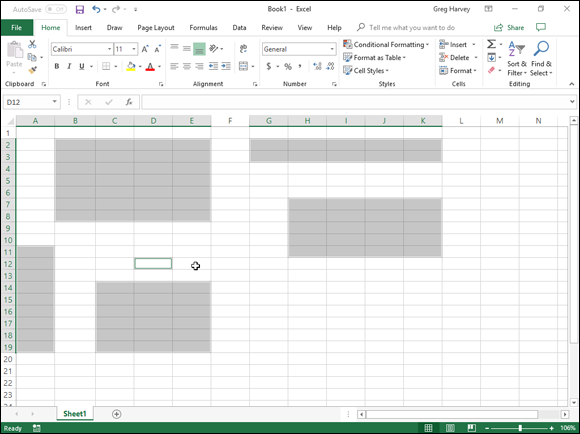
FIGURE 3-1: Several cell selections of various shapes and sizes.
In Excel, you can select more than one cell range at a time (a phenomenon somewhat ingloriously called a noncontiguous or nonadjacent selection). In fact, although Figure 3-1 appears to contain several cell selections, it’s really just one big, nonadjacent cell selection with cell D12 (the active one) as the cell that was selected last.
Point-and-click cell selections
A mouse (provided that the device you’re running Excel 2019 on has a mouse) is a natural for selecting a range of cells. Just position the mouse pointer (in its thick, white cross form) on the first cell and then click and drag in the direction that you want to extend the selection.
- To extend the cell selection to columns to the right, drag your mouse to the right, highlighting neighboring cells as you go.
- To extend the selection to rows to the bottom, drag your mouse down.
- To extend the selection down and to the right at the same time, drag your mouse diagonally toward the cell in the lower-right corner of the block you’re highlighting.
Shifty cell selections
To speed up the old cell-selection procedure, you can use the Shift+click method, which goes as follows:
-
Click the first cell in the selection.
This selects that cell.
-
Position the mouse pointer in the last cell in the selection.
This is kitty-corner from the first cell in your selected rectangular block.
-
Press the Shift key and hold it down while you click the mouse button again.
When you click the mouse button the second time, Excel selects all the cells in the columns and rows between the first cell and last cell.
The Shift key works with the mouse like an extend key to extend a selection from the first object you select through to, and including, the second object you select. See the section “Extend that cell selection,” later in this chapter. Using the Shift key enables you to select the first and last cells, as well as all the intervening cells in a worksheet or all the document names in a list.
If, when making a cell selection with the mouse, you notice that you include the wrong cells before you release the mouse button, you can deselect the cells and resize the selection by moving the pointer in the opposite direction. If you already released the mouse button, click the first cell in the highlighted range to select just that cell (and deselect all the others) and then start the whole selection process again.
Adding to and subtracting from cell selections
To select a nonadjacent cell selection made up of more than one nontouching block of cells, drag through the first cell range and release the mouse button. Then hold down the Ctrl key while you click the first cell of the second range and drag the pointer through the cells in this range. As long as you hold down Ctrl while you select the subsequent ranges, Excel doesn’t deselect any of the previously selected cell ranges.
The Ctrl key can work with the mouse like an add or subtract key in Excel 2019. As an add key, you use it to include non-neighboring objects in the current worksheet. See the section “Nonadjacent cell selections with the keyboard,” later in this chapter. By using the Ctrl key, you can add to the selection of cells in a worksheet or to the document names in a list without having to deselect those already selected.
 To use the Ctrl key to deselect a range of cells
within the current cell selection, hold down the Ctrl key and drag
through the range that you want to deselect (subtract from the
selected range) before releasing the mouse button and Ctrl key.
To use the Ctrl key to deselect a range of cells
within the current cell selection, hold down the Ctrl key and drag
through the range that you want to deselect (subtract from the
selected range) before releasing the mouse button and Ctrl key.
Touchy-feely cell selections
If you’re running Excel 2019 on a touchscreen
device such as a Windows tablet (like the Microsoft Surface Pro) or
a computer (such as the Surface Laptop), you simply use your finger
or stylus to make your cell selections. Simply tap the first cell
in the selection (the equivalent of clicking with a mouse) and then
drag the selection handle (one of the two circles that appears in
the upper-left and lower-right corner of the cell) through the rest
of the adjacent cells to extend the cell selection and select the
entire range.
 Keep in mind that you can select only
one range at a time on a touchscreen when you’re dragging through
the cells directly on the screen with your finger or a stylus. The
Shift and Ctrl key range selection and extender techniques
(discussed in the previous two sections) only work when dragging
through cells indirectly with a mouse or on a computer touchpad
using the Shift and Ctrl keys on a physical keyboard.
Keep in mind that you can select only
one range at a time on a touchscreen when you’re dragging through
the cells directly on the screen with your finger or a stylus. The
Shift and Ctrl key range selection and extender techniques
(discussed in the previous two sections) only work when dragging
through cells indirectly with a mouse or on a computer touchpad
using the Shift and Ctrl keys on a physical keyboard.
Going for the “big” cell selections
You can select the cells in entire columns or rows or even all the cells in the worksheet by applying the following clicking-and-dragging techniques to the worksheet frame:
- To select every single cell in a particular column, click its column letter on the frame at the top of the worksheet document window.
- To select every cell in a particular row, click its row number on the frame at the left edge of the document window.
- To select a range of entire columns or rows, drag through the column letters or row numbers on the frame surrounding the workbook.
- To select more than entire columns or rows that are not right next to each other (that old noncontiguous stuff, again), press and hold down the Ctrl key while you click the column letters or row numbers of the columns or rows that you want to add to the selection.
-
To select every cell in the worksheet, press
Ctrl+A or click the Select All button, which is the button with the
triangle pointing downward on the diagonal (which reminds me of the
corner of a dog-eared book page). It’s in the upper-left corner of
the workbook frame, formed by the intersection of the row with the
column letters and the column with the row numbers.
Selecting the cells in a table of data, courtesy of AutoSelect
Excel provides a quick way (called AutoSelect) to select all the cells in a table of data entered as a solid block with your mouse. To use AutoSelect, simply follow these steps:
-
Click the first cell of the table to select it.
This is the cell in the table’s upper-left corner.
-
Hold down the Shift key while you double-click the right or bottom edge of the selected cell with the arrowhead mouse pointer (see Figure 3-2).
Double-clicking the bottom edge of the cell causes the cell selection to expand to the cell in the last row of the first column (as shown in Figure 3-3). If you double-click the right edge of the cell, the cell selection expands to the cell in the last column of the first row.
3a. Double-click somewhere on the
right edge of the cell selection (refer to Figure 3-3) if the cell selection now
consists of the first column of the table.
This selects all the remaining rows of the table of data (as shown
in Figure 3-4).
3b. Double-click somewhere on the
bottom edge of the current cell selection if the cell selection now
consists of the first row of the table.
This selects all the remaining rows in the table.
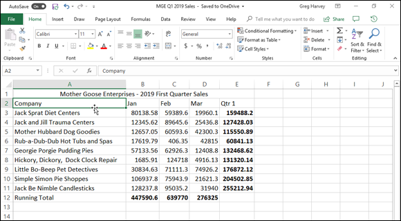
FIGURE 3-2: Position the mouse pointer on the first cell’s bottom edge to select all cells of the table’s first column.
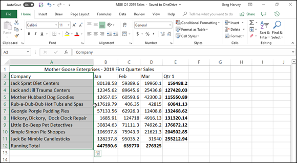
FIGURE 3-3: Hold down Shift while you double-click the bottom edge of the first cell to extend the selection down the column.
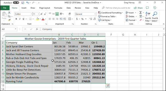
FIGURE 3-4: Hold down Shift as you double-click the right edge of the current selection to extend it across the rows of the table.
Although the preceding steps may lead you to
believe that you have to select the first cell of the table when
you use AutoSelect, you can actually select any of the cells in the
four corners of the table. Then, when expanding the cell selection
in the table with the Shift key depressed, you can choose whatever
direction you like to either select the first or last row of the
table or the first or last column. (Choose left, by clicking the
left edge; right, by clicking the right edge; up, by clicking the
top edge; or down, by clicking the bottom edge.) After expanding
the cell selection to include either the first or last row or first
or last column, you need to click whichever edge of that current
cell selection that will expand it to include all the remaining
table rows or columns.
Keyboard cell selections
If you’re not keen on using the mouse, you can use the keyboard to select the cells you want. Sticking with the Shift+click method of selecting cells, the easiest way to select cells with the keyboard is to combine the Shift key with other keystrokes that move the cell cursor. (I list these keystrokes in Chapter 1.)
Start by positioning the cell cursor in the first cell of the selection and then holding the Shift key while you press the appropriate cell pointer movement keys. When you hold the Shift key while you press direction keys — such as the arrow keys (↑, →, ↓, ←), PgUp, or PgDn — Excel anchors the selection on the current cell, moves the cell cursor, and highlights cells as it goes.
When making a cell selection this way, you can
continue to alter the size and shape of the cell range with the
cell pointer movement keys as long as you don’t release the Shift
key. After you release the Shift key, pressing any of the cell
pointer movement keys immediately collapses the selection, reducing
it to just the cell with the cell cursor.
Extend that cell selection
If holding the Shift key while you move the cell cursor is too tiring, you can place Excel in Extend mode by pressing (and promptly releasing) F8 before you press any cell pointer movement key. Excel displays the Extend Selection indicator on the left side of the Status bar — when you see this indicator, the program will select all the cells that you move the cell cursor through (just as though you were holding down the Shift key).
After you highlight all the cells you want in the cell range, press F8 again (or Esc) to turn off Extend mode. The Extend Selection indicator disappears from the Status bar, and then you can once again move the cell cursor with the keyboard without highlighting everything in your path. In fact, when you first move the pointer, all previously selected cells are deselected.
AutoSelect keyboard style
For the keyboard equivalent of AutoSelect with the mouse (see the “Selecting the cells in a table of data, courtesy of AutoSelect” section), you combine the use of the F8 key (Extend key) or the Shift key with the Ctrl+arrow keys or End+arrow keys to zip the cell cursor from one end of a block to the other and merrily select all the cells in that path.
To select an entire table of data with a keyboard version of AutoSelect, follow these steps:
-
Position the cell cursor in the first cell.
That’s the cell in the upper-left corner of the table.
- Press F8 (or hold the Shift key) and then press Ctrl+ → to extend the cell selection to the cells in the columns on the right.
- Then press Ctrl+↓ to extend the selection to the cells in the rows below.
The directions in the preceding steps
are somewhat arbitrary — you can just as well press Ctrl+↓ before
you press Ctrl+ →. Just be sure (if you’re using the Shift key
instead of F8) that you don’t let up on the Shift key until after
you finish performing these two directional maneuvers. Also, if you
press F8 to get the program into Extend mode, don’t forget to press
this key again to get out of Extend mode after the table cells are
all selected, or you’ll end up selecting cells that you don’t want
included when you next move the cell cursor.
Nonadjacent cell selections with the keyboard
Selecting more than one cell range is a little more complicated with the keyboard than it is with the mouse. When using the keyboard, you alternate between anchoring the cell cursor and moving it to select the cell range and unanchoring the cell cursor and repositioning it at the beginning of the next range. To unanchor the cell cursor so that you can move it into position for selecting another range, press Shift+F8. This puts you in Add to Selection mode, in which you can move to the first cell of the next range without selecting any more cells. Excel lets you know that the cell cursor is unanchored by displaying the Add to Selection indicator on the left side of the Status bar.
To select more than one cell range by using the keyboard, follow these general steps:
- Move the cell cursor to the first cell of the first cell range that you want to select.
-
Press F8 to get into Extend Selection mode.
Move the cell cursor to select all the cells in the first cell range. Alternatively, hold the Shift key while you move the cell cursor.
-
Press Shift+F8 to switch from Extend Selection mode to Add to Selection mode.
The Add to Selection indicator appears in the Status bar.
- Move the cell cursor to the first cell of the next nonadjacent range that you want to select.
- Press F8 again to get back into Extend Selection mode and then move the cell cursor to select all the cells in this new range.
- If you still have other nonadjacent ranges to select, repeat Steps 3, 4, and 5 until you select and add all the cell ranges that you want to use.
Cell selections à la Go To
If you want to select a large cell range that would take a long time to select by pressing various cell pointer movement keys, use the Go To feature to extend the range to a far distant cell. All you gotta do is follow this pair of steps:
- Position the cell cursor in the first cell of the range and then press F8 to anchor the cell cursor and get Excel into Extend Selection mode.
- Press F5 or Ctrl+G to open the Go To dialog box, type the address of the last cell in the range (the cell kitty-corner from the first cell), and then click OK or press Enter.
Because Excel is in Extend Selection
mode at the time you use the Go To feature to jump to another cell,
the program not only moves the cell cursor to the designated cell
address but selects all the intervening cells as well. After
selecting the range of cells with the Go To feature, don’t forget
to press F8 (the Extend Selection key) again to prevent the program
from messing up your selection by adding more cells the next time
you move the cell cursor.
Using the Format as Table Gallery
Here’s a formatting technique that doesn’t require you to do any prior cell selecting. (Kinda figures, doesn’t it?) The Format as Table feature is so automatic that the cell cursor just has to be within the table of data prior to you clicking the Format as Table command button in the Styles group on the Home tab. Clicking the Format as Table command button opens its rather extensive Table Styles gallery with the formatting thumbnails divided into three sections — Light, Medium, and Dark — each of which describes the intensity of the colors used by its various formats.
As soon as you click one of the table formatting thumbnails in this Table Styles gallery, Excel makes its best guess as to the cell range of the data table to apply it to (indicated by the marquee around its perimeter), and the Format As Table dialog box, similar to the one shown in Figure 3-5, appears.
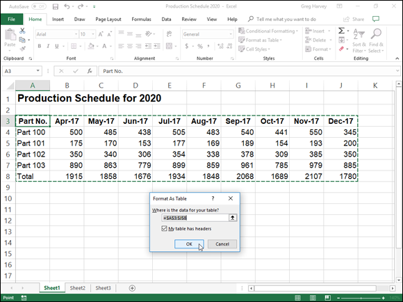
FIGURE 3-5: Selecting a format from the Table Styles gallery and indicating its range in the Format As Table dialog box.
This dialog box contains a Where Is the Data for Your Table text box that shows the address of the cell range currently selected by the marquee and a My Table Has Headers check box.
If Excel does not correctly guess the range of the data table you want to format, drag through the cell range to adjust the marquee and the range address in the Where Is the Data for Your Table text box. If your data table doesn’t use column headers or, if the table has them, but you still don’t want Excel to add Filter drop-down buttons to each column heading, deselect the My Table Has Headers check box before you click the OK button.
 The table formats in the Table Styles gallery
are not available if you select multiple nonadjacent cells before
you click the Format as Table command button on the Home tab.
The table formats in the Table Styles gallery
are not available if you select multiple nonadjacent cells before
you click the Format as Table command button on the Home tab.
After you click the OK button in the Format As Table dialog box, Excel applies the formatting of the thumbnail you clicked in the gallery to the data table. Additionally, the Design tab appears under the Table Tools contextual tab at the end of the Ribbon, and the table is selected with the Quick Analysis tool appearing in the lower-right corner, as shown in Figure 3-6.

FIGURE 3-6: After you select a format from the Table Styles gallery, the Design tab appears under the Table Tools contextual tab.
The Design tab enables you to use Live Preview to
see how your table would appear. Simply click the Table Styles
continuation button on the Design tab of the Ribbon (or Quick
Styles button, if it’s displayed) and then position the mouse
pointer over any of the format thumbnails in the Table Styles
drop-down palette to see the data in your table appear in that
table format. Click the button with the triangle pointing downward
to scroll up new rows of table formats in the Table Styles group;
click the button with the triangle pointing upward to scroll down
rows without opening the Table Styles gallery and possibly
obscuring the actual data table in the Worksheet area. Click the
More button (the one with the horizontal bar above the
downward-pointing triangle) to redisplay the Table gallery and then
mouse over the thumbnails in the Light, Medium, and Dark sections
to have Live Preview apply them to the table.
Whenever you assign a format in the Table Styles gallery to one of the data tables in your workbook, Excel automatically assigns that table a generic range name (Table1, Table2, and so on). You can use the Table Name text box in the Properties group on the Design tab to rename the data table to give it a more descriptive range name. (See Chapter 6 for all you need to know about naming cell ranges.)
You can also use the Tables option on
the Quick Analysis tool to format your worksheet data as a table.
Simply select the table data (including headings) as a cell range
in the worksheet and then click the Tables option on the Quick
Analysis tool, followed by the Table option below at the very
beginning of the Tables options. Excel then assigns the Table Style
Medium 9 style to your table while at same time selecting the Design tab on the Ribbon. Then if you’re
not too keen on this table style, you can use Live Preview in the
Tables Styles gallery on this tab to find the table formatting that
you do want to use.
Customizing table formats
In addition to enabling you to select a new format from the Table Styles gallery, the Design tab contains a Table Style Options group containing a bunch of check boxes that enable you to customize the look of the selected table format even further:
- Header Row to display the top row with the labels that identify the type of data in each column as well as the Filter buttons for sorting and filtering data in the first row of the table. (This check box is selected by default.)
- Total Row to have Excel add a Total Row to the bottom of the table that displays the sums of each column that contains values. To apply another Statistical function to the values in a particular column, click the cell in that column’s Total Row to display a drop-down list button and then select the function — Average, Count, Count Numbers, Max, Min, Sum, StdDev (Standard Deviation), or Var (Variance).
- Banded Rows to have Excel apply shading to every other row in the table.
- First Column to have Excel display the row headings in the first column of the table in bold.
- Last Column to have Excel display the row headings in the last column of the table in bold.
- Banded Columns to have Excel apply shading to every other column in the table.
- Filter Button to have Excel display drop-down buttons to the right of the entries when the table’s Header Row is displayed that you can use to sort and filter the data in that column. (This check box is selected by default.)
When you finish selecting and/or customizing the formatting of your data table, click a cell outside of the table to remove the Table Tools contextual tab (with its Design tab) from the Ribbon. If later, you decide that you want to further experiment with the table’s formatting, click any of the table’s cells to redisplay the Table Tools’ Design tab at the end of the Ribbon.
Creating a new custom Table Style
Excel 2019 lets you create your own custom styles to add to the Tables Styles gallery and use in formatting your worksheet tables. Once created, a custom Table Style not only applies just the kind of formatting you want for your worksheet tables but can also be reused on tables of data in any worksheet you create or edit in the future. You can even designate one of the custom styles you create as the new Table Style default for your workbook so that it’s automatically applied when you later format a data table in its worksheets with the Tables option on the Quick Analysis toolbar.
To create a custom Table Style, you follow these steps:
- Format the data in your worksheet as a table using one of the existing styles (as described in the previous section).
-
On the Design contextual tab of the Tables Tool tab, click the Table Styles More drop-down button and then select the New Table Style option near the bottom of the gallery.
The New Table Style dialog box, shown in Figure 3-7, appears.
- Replace the generic, table style name, Table Style 1, with a more descriptive name in the Name text box.
-
Modify each of the individual table components in the Table Elements list box (from Whole Table through Last Total Cell) with the custom formatting you want included in your new custom table style.
To customize the formatting for a table element, select its name in the Table Element list box. After you select the element, click the Format button to open the Format Cells dialog box where you can change that element’s font style and/or color on its Font tab, the border style and/or color on its Border tab, or the fill effect and/or color on its Fill tab. (See the “Futzing with the Fonts,” “Bring on the borders!,” and “Applying fill colors, patterns, and gradient effects to cells” sections later in this chapter for details on adjusting these different formats.)
Note that when customizing a First or Second Column or Row Stripe element (that controls the shading or banding of table’s column or row), in addition to changing the fill for the banding on the Fill tab of the Format Cells dialog box, you can also increase how many columns or rows are banded by increasing the number in the Stripe Size drop-down list that appears when you select one of the Stripe elements.
As you assign new formatting to a particular table element, Excel displays a description of the formatting change below the Element Formatting heading of New Table Style dialog box, as long as that table element remains selected in the Table Element list box. When you add a new fill color to a particular element, this color appears in the Preview area of this dialog box regardless of which component is selected in the Table Element list box.
- (Optional) If you want your new custom table style to become the default table style for all the data tables you format in your workbook, select the Set as Default Table Style for This Document check box.
- Click the OK button to save the settings for your new custom table style and close the New Table Style dialog box.

FIGURE 3-7: Use the options in the New Table Style dialog box to create a new custom table style to add to the Table Styles gallery.
As soon as you close the New Table Style dialog box, a thumbnail of the new custom table style you just created appears at the very beginning of the truncated Table Styles gallery that appears on the Design tab of the Table Tools font. You can then apply the newly created style to the currently selected table of data (the sample table you formatting in order to create the new style) by clicking this thumbnail. When you next open the entire Table Styles gallery to format other tables of data that you add to your worksheets, the thumbnail of the custom style you created will appear in its own Custom section at the very top of the gallery.
If you made changes to the fill formatting for
the First or Second Column Stripe element in the custom table
style, don’t forget to select the Banded Rows check box in Table
Styles Options section on the Table Tools Design tab to make it
appear in the formatted data table. So, too, if you made changes to
the First or Second Row Stripe, you need to select the Banded Rows
check box to make these formats appear.
To further modify, copy (in order to use its settings as the basis for a new custom style), delete, or add a custom style to the Quick Analysis toolbar, right-click its thumbnail image in the Table Styles gallery and then choose the Modify, Duplicate, Delete, or Add Gallery to Quick Access Toolbar option on its context menu.
Cell Formatting from the Home Tab
Some spreadsheet tables or ranges within them require a lighter touch than the Format as Table command button offers. For example, you may have a data table where the only emphasis you want to add is to make the column headings bold at the top of the table and to underline the row of totals at the bottom (done by drawing a borderline along the bottom of the cells).
The formatting buttons that appear in the Font, Alignment, and Number groups on the Home tab enable you to accomplish just this kind of targeted cell formatting. See Table 3-1 for a complete rundown on how to use each of these formatting buttons.
TABLE 3-1 Formatting Command Buttons in the Font, Alignment, and Number Groups on the Home Tab
|
Group |
Button Name |
Function |
|
Font |
||
|
Font |
Displays a Font drop-down menu from which you can select a new font for your cell selection |
|
|
Font Size |
Displays a Font Size drop-down menu from which you can select a new font size for your cell selection — click the Font Size text box and enter the desired point size if it doesn’t appear on the drop-down menu |
|
|
Increase Font Size |
Increases the current font size of the cell selection (as it appears in the Font Size drop-down list box) by one point |
|
|
Decrease Font Size |
Decreases the current font size of the cell selection (as it appears in the Font Size drop-down list box) by one point |
|
|
Bold |
Applies boldface to the entries in the cell selection |
|
|
Italic |
Italicizes the entries in the cell selection |
|
|
Underline |
Underlines the entries in the cell selection |
|
|
Borders |
Displays a Borders drop-down menu from which you can select a border style for the cell selection |
|
|
Fill Color |
Displays a Color drop-down palette from which you can select a new background color for the cell selection |
|
|
Font Color |
Displays a Color drop-down palette from which you can select a new font color for the cell selection |
|
|
Alignment |
||
|
Align Left |
Aligns all the entries in the cell selection with the left edge of their cells |
|
|
Center |
Centers all the entries in the cell selection within their cells |
|
|
Align Right |
Aligns all the entries in the cell selection with the right edge of their cells |
|
|
Decrease Indent |
Decreases the margin between entries in the cell selection and their left cell borders by about one character width |
|
|
Increase Indent |
Increases the margin between the entries in the cell selection and their left cell borders by about one character width |
|
|
Top Align |
Aligns the entries in the cell selection with the top border of their cells |
|
|
Middle Align |
Vertically centers the entries in the cell selection between the top and bottom borders of their cells |
|
|
Bottom Align |
Aligns the entries in the cell selection with the bottom border of their cells |
|
|
Orientation |
Displays a drop-down menu with options for changing the angle and direction of the entries in the cell selection |
|
|
Wrap Text |
Wraps the entries in the cell selection that spill over their right borders onto multiple lines within the current column width |
|
|
Merge & Center |
Merges the cell selection into a single cell and centers the entry in the first cell between its new left and right border — click the Merge and Center drop-down button to display a menu of options that enable you to merge the cell selection into a single cell without centering the entries, as well as to split up a merged cell back into its original individual cells |
|
|
Number |
||
|
Number Format |
Displays the number format applied to the active cell in the cell selection — click its drop-down button to display a menu showing the active cell in cell selection formatted with all of Excel’s major number formats |
|
|
Accounting Number Format |
Formats the cell selection using the Accounting number format that adds a dollar sign, uses commas to separate thousands, displays two decimal places, and encloses negative values in a closed pair of parentheses — click the Accounting Number Format’s drop-down button to display a menu of other major Currency number formats from which you can choose |
|
|
Percent Style |
Formats the cell selection using the Percentage number format that multiplies the values by 100 and adds a percent sign with no decimal places |
|
|
Comma Style |
Formats the cell selection with the Comma Style number format that uses commas to separate thousands, displays two decimal places, and encloses negative values in a closed pair of parentheses |
|
|
Increase Decimal |
Adds a decimal place to the values in the cell selection |
|
|
Decrease Decimal |
Removes a decimal place from the values in the cell selection |
Don’t forget about the tooltips that
appear when you highlight one of these formatting command buttons
with your mouse or Touch pointer. These tooltips not only give you
a short description of the button’s function, but also display any
shortcut keys for quickly adding or removing attributes from the
entries in the cell selection.
Formatting Cells Close to the Source with the Mini-bar
Excel 2019 makes it easy to apply common formatting changes to a cell selection right within the Worksheet area thanks to the mini-toolbar feature, nicknamed the mini-bar (makes me thirsty just thinking about it!).
To display the mini-bar, select the cells that need formatting and then right-click somewhere in the cell selection. The cell range’s context menu along with the mini-bar then appears near the cell selection. When you select a tool in the mini-bar, such as Font or Font Size pop-up button, the context menu disappears (see Figure 3-8).
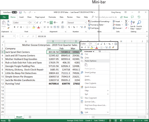
FIGURE 3-8: Use the buttons on the mini-bar to apply common formatting changes to the cell selection within the Worksheet area.
As you can see in this figure, the mini-bar contains most of the buttons from the Font group of the Home tab (with the exception of the Underline button). It also contains the Center and Merge & Center buttons from the Alignment group (see the “Altering the Alignment” section, later in this chapter) and the Accounting Number Format, Percent Style, Comma Style, Increase Decimal, and Decrease Decimal buttons from the Number group (see the “Understanding the number formats” section, later in this chapter). Simply click these buttons to apply their formatting to the current cell selection.
Additionally, the mini-bar contains the Format Painter button from the Clipboard group of the Home tab that you can use to copy the formatting in the active cell to a cell selection you make (see the “Fooling Around with the Format Painter” section, later in this chapter for details).
Using the Format Cells Dialog Box
Although the command buttons in the Font, Alignment, and Number groups on the Home tab give you immediate access to the most commonly used formatting commands, they do not represent all of Excel’s formatting commands by any stretch of the imagination.
To have access to all the formatting commands, you need to open the Format Cells dialog box shown in Figure 3-9 by doing any of the following:
- Click the More Number Formats option at the very bottom of the drop-down menu attached to the Number Format button.
- Click the Number Format Dialog Box launcher in the lower right of the Number group.
- Press Ctrl+1.

FIGURE 3-9: The Format Cells dialog box gives you access to a wide range of format settings to apply to the selected cell range.
As you can see in Figure 3-9, the Format Cells dialog contains six tabs: Number, Alignment, Font, Border, Fill, and Protection. In this chapter, I show you how to use them all except the Protection tab. For information on that tab, see Chapter 6.
The keystroke shortcut that opens the Format
Cells dialog box — Ctrl+1 — is one worth knowing. Just press the
Ctrl key plus the number 1 key, and not the function
key F1.
Understanding the number formats
As I explain in Chapter 2, how you enter values into a worksheet determines the type of number format that they get. Here are some examples:
- If you enter a financial value complete with the dollar sign and two decimal places, Excel assigns a Currency number format to the cell along with the entry.
- If you enter a value representing a percentage as a whole number followed by the percent sign without any decimal places, Excel assigns the cell the Percentage number format that follows this pattern along with the entry.
- If you enter a date (dates are values, too) that follows one of the built-in Excel number formats, such as 11/06/13 or 06-Nov-13, the program assigns a Date number format that follows the pattern of the date along with a special value representing the date.
Although you can format values in this manner as you go along (which is necessary in the case of dates), you don’t have to do it this way. You can always assign a number format to a group of values before or after you enter them. Formatting numbers after you enter them is often the most efficient way to go because it’s just a two-step procedure:
- Select all the cells containing the values that need dressing up.
- Select the number format that you want to use from the formatting command buttons on the Home tab or the options available on the Number tab in the Format Cells dialog box.
Even if you’re a really, really good typist and
prefer to enter each value exactly as you want it to appear in the
worksheet, you still have to resort to using number formats to make
the values that are calculated by formulas match the others you
enter. This is because Excel applies a General number format (which
the Format Cells dialog box defines: “General format cells have no
specific number format.”) to all the values it calculates, as well
as any you enter that don’t exactly follow one of the other Excel
number formats. The biggest problem with the General format is that
it has the nasty habit of dropping all leading and trailing zeros
from the entries. This makes it very hard to line up numbers in a
column on their decimal points.
You can view this sad state of affairs in Figure 3-10, which is a sample worksheet with the first-quarter 2019 sales figures for Mother Goose Enterprises before any of the values have been formatted. Notice how the decimal in the numbers in the monthly sales figures columns zig and zag because they aren’t aligned on the decimal place. This is the fault of Excel’s General number format; the only cure is to format the values with a uniform number format.

FIGURE 3-10: Numbers with decimals don’t align when you choose General formatting.
Accounting for the dollars and cents in your cells
Given the financial nature of most worksheets, you probably use the Accounting number format more than any other. Applying this format is easy because you can assign it to the cell selection simply by clicking the Accounting Number Format button on the Home tab.
The Accounting number format adds a
dollar sign, commas between thousands of dollars, and two decimal
places to any values in a selected range. If any of the values in
the cell selection are negative, this number format displays them
in parentheses (the way accountants like them). If you want a minus
sign in front of your negative financial values rather than
enclosing them in parentheses, select the Currency format on the
Number Format drop-down menu or on the Number tab of the Format
Cells dialog box.
You can see in Figure 3-11 that only the cells containing totals are selected (cell ranges E3:E10 and B10:D10). This cell selection was then formatted with the Accounting number format by simply clicking its command button (the one with the $ icon, naturally) in the Number group on the Ribbon’s Home tab.

FIGURE 3-11: The totals in the Mother Goose sales table after clicking the Accounting Number Format button on the Home tab.
Although you could put all the figures in the
table into the Accounting number format to line up the decimal
points, this would result in a superabundance of dollar signs in a
fairly small table. In this example, I only formatted the monthly
and quarterly totals with the Accounting number format.
“Look, Ma, no more format overflow!”
When I apply the Accounting number format to the selection in the cell ranges of E3:E10 and B10:D10 in the sales table shown in Figure 3-11, Excel adds dollar signs, commas between the thousands, a decimal point, and two decimal places to the highlighted values. At the same time, Excel automatically widens columns B, C, D, and E just enough to display all this new formatting. In versions of Excel earlier than Excel 2003, you had to widen these columns yourself, and instead of the perfectly aligned numbers, you were confronted with columns of #######s in cell ranges E3:E10 and B10:D10. Such pound signs (where nicely formatted dollar totals should be) serve as overflow indicators, declaring that whatever formatting you added to the value in that cell has added so much to the value’s display that Excel can no longer display it within the current column width.
Fortunately, Excel eliminates the format overflow indicators when you’re formatting the values in your cells by automatically widening the columns. The only time you’ll ever run across these dreaded #######s in your cells is when you take it upon yourself to narrow a worksheet column manually (see the section “Calibrating Columns,” later in this chapter) to the extent that Excel can no longer display all the characters in its cells with formatted values.
Currying your cells with the Comma Style
The Comma Style format offers a good alternative to the Currency format. Like Currency, the Comma Style format inserts commas in larger numbers to separate thousands, hundred thousands, millions, and … well, you get the idea.
This format also displays two decimal places and puts negative values in parentheses. What it doesn’t display is dollar signs. This makes it perfect for formatting tables where it’s obvious that you’re dealing with dollars and cents or for larger values that have nothing to do with money.
The Comma Style format also works well for the bulk of the values in the sample first-quarter sales worksheet. Check out Figure 3-12 to see this table after I format the cells containing the monthly sales for all the Mother Goose Enterprises with the Comma Style format. To do this, select the cell range B3:D9 and click the Comma Style button — the one with the comma icon (,) — in the Number group on the Home tab.

FIGURE 3-12: Monthly sales figures after formatting cells with the Comma Style number format.
Note how, in Figure 3-12, the Comma Style format takes care of the earlier decimal alignment problem in the quarterly sales figures. Moreover, Comma Style–formatted monthly sales figures align perfectly with the Currency format–styled monthly totals in row 10. If you look closely (you may need a magnifying glass for this one), you see that these formatted values no longer abut the right edges of their cells; they’ve moved slightly to the left. The gap on the right between the last digit and the cell border accommodates the right parenthesis in negative values, ensuring that they, too, align precisely on the decimal point.
Playing around with Percent Style
Many worksheets use percentages in the form of interest rates, growth rates, inflation rates, and so on. To insert a percentage in a cell, type the percent sign (%) after the number. To indicate an interest rate of 12 percent, for example, you enter 12% in the cell. When you do this, Excel assigns a Percentage number format and, at the same time, divides the value by 100 (that’s what makes it a percentage) and places the result in the cell (0.12 in this example).
Not all percentages in a worksheet are entered by hand in this manner. Some may be calculated by a formula and returned to their cells as raw decimal values. In such cases, you should add a Percent format to convert the calculated decimal values to percentages (done by multiplying the decimal value by 100 and adding a percent sign).
The sample first-quarter-sales worksheet just happens to have some percentages calculated by formulas in row 12 that need formatting (these formulas indicate what percentage each monthly total is of the first-quarter total in cell E10). In Figure 3-13, these values reflect Percent Style formatting. To accomplish this feat, you simply select the cells and click the Percent Style button in the Number group on the Home tab. (Need I point out that it’s the button with the % symbol?)
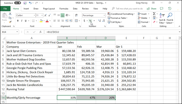
FIGURE 3-13: Monthly-to-quarterly sales percentages with Percentage number formatting.
Deciding how many decimal places
You can increase or decrease the number of decimal places used in a number entered by using the Accounting Number Format, Comma Style, or Percent Style button in the Number group of the Home tab simply by clicking the Increase Decimal button or the Decrease Decimal button in this group. Each time you click the Increase Decimal button (the one with the arrow pointing left), Excel adds another decimal place to the number format you apply.
The values behind the formatting
Make no mistake about it — all that these fancy number formats do is spiff up the presentation of the values in the worksheet. Like a good illusionist, a particular number format sometimes appears to transform some entries, but in reality, the entries are the same old numbers you started with. For example, suppose that a formula returns the following value:
25.6456
Now suppose that you format the cell containing this value with the Accounting Number Format button on the Home tab. The value now appears as follows:
$25.65
This change may lead you to believe that Excel rounded the value up to two decimal places. In fact, the program has rounded up only the display of the calculated value — the cell still contains the same old value of 25.6456. If you use this cell in another worksheet formula, Excel uses the behind-the-scenes value in its calculation, not the spiffed-up one shown in the cell.
If you want the values to match their
formatted appearance in the worksheet, Excel can do that in a
single step. Be forewarned, however, that this is a one-way trip.
You can convert all underlying values to the way they are displayed
by selecting a single check box, but you can’t return them to their
previous state by deselecting this check box.
Well, because you insist on knowing this little trick anyway, here goes (just don’t write and try to tell me that you weren’t warned):
-
Make sure that you format all the values in your worksheet with the correct number of decimal places.
You must do this step before you convert the precision of all values in the worksheet to their displayed form.
- Click File ⇒ Options ⇒ Advanced or press Alt+FTA to open the Advanced tab of the Excel Options dialog box.
-
In the When Calculating This Workbook section, select the Set Precision as Displayed check box (to fill it with a check mark).
Excel displays the Data Will Permanently Lose Accuracy alert dialog box.
- Go ahead (live dangerously) and click the OK button or press Enter to convert all values to match their display. Click OK again to close the Excel Options dialog box.
Save the workbook with the calculated values.
After converting all the values in a worksheet by selecting the Set
Precision as Displayed check box, open the Save As dialog box
(select File ⇒ Save As or press Alt+FA). Edit the filename in the
File Name text box (maybe by appending as Displayed to the
current filename) before you click the Save button or press Enter.
That way, you’ll have two copies: the original workbook file with
the values as entered and calculated by Excel and the new as
Displayed version.
Make it a date!
In Chapter 2, I mention that you can easily create formulas that calculate the differences between the dates and times that you enter in your worksheets. The only problem is that when Excel subtracts one date from another date or one time from another time, the program automatically formats the calculated result in a corresponding date or time number format as well. For example, if you enter 8-15-19 in cell B4 and 4/15/19 in cell C4 and in cell D4 enter the following formula for finding the number of elapsed days between the two dates:
=B4-C4
Excel correctly returns the result of 122 (days) using the General number format. However, when dealing with formulas that calculate the difference between two times in a worksheet, you have to reformat the result that appears in a corresponding time format into the General format. For example, suppose that you enter 8:00 AM in cell B5 and 4:00 PM in cell C5 and then create in cell D5 the following formula for calculating the difference in hours between the two times:
=C5-B5
You then have to convert the result in cell D5 — that automatically appears as 8:00 AM — to the General format. When you do this, the fraction 0.333333 — representing its fraction of the total 24-hour period — replaces 8:00 AM in cell D5. You can then convert this fraction of a total day into the corresponding number of hours by multiplying this cell by 24 and formatting the cell with the General format.
Ogling some of the other number formats
Excel supports more number formats than just the Accounting, Comma Style, and Percentage number formats. To use them, select the cell range (or ranges) you want to format and select Format Cells on the cell shortcut menu (right-click somewhere in the cell selection to activate this menu) or just press Ctrl+1 to open the Format Cells dialog box.
After the Format Cells dialog box opens with the Number tab displayed, you select the desired format from the Category list box. Some number formats — such as Date, Time, Fraction, and Special — give you further formatting choices in a Type list box. Other number formats, such as Number and Currency, have their own particular boxes that give you options for refining their formats. When you click the different formats in these list boxes, Excel shows what effect this would have on the first of the values in the current cell selection in the Sample area above. When the sample has the format that you want to apply to the current cell selection, you just click OK or press Enter to apply the new number format.
Excel contains a nifty category of number formats called Special. The Special category contains the following four number formats that may interest you:
- Zip Code: Retains any leading zeros in the value (important for zip codes and of absolutely no importance in arithmetic computations). Example: 00123.
- Zip Code + 4: Automatically separates the last four digits from the first five digits and retains any leading zeros. Example: 00123-5555.
- Phone Number: Automatically encloses the first three digits of the number in parentheses and separates the last four digits from the previous three with a dash. Example: (999) 555-1111.
- Social Security Number: Automatically puts dashes in the value to separate its digits into groups of three, two, and four. Example: 666-00-9999.
These Special number formats really come in handy when creating data lists in Excel that often deal with stuff like zip codes, telephone numbers, and sometimes even Social Security numbers (see Chapter 11 for more on creating and using data lists).
Calibrating Columns
For those times when Excel 2019 doesn’t automatically adjust the width of your columns to your complete satisfaction, the program makes changing the column widths a breeze. The easiest way to adjust a column is to do a best-fit, using the AutoFit feature. With this method, Excel automatically determines how much to widen or narrow the column to fit the longest entry currently in the column.
Here’s how to use AutoFit to get the best fit for a column:
-
Position the mouse on the right border of the worksheet frame with the column letter at the top of the worksheet.
The pointer changes to a double-headed arrow pointing left and right.
-
Double-click the mouse button.
Excel widens or narrows the column width to suit the longest entry.
You can apply a best-fit to more than one column at a time. Simply select all the columns that need adjusting (if the columns neighbor one another, drag through their column letters on the frame; if they don’t, Ctrl+click the individual column letters). After you select the columns, double-click any of the right borders on the frame.
Best-fit à la AutoFit doesn’t always produce the expected results. A long title that spills into several columns to the right produces a very wide column when you use best-fit.
When AutoFit’s best-fit won’t do, drag the right
border of the column (on the frame) until it’s the size you need
instead of double-clicking it. This manual technique for
calibrating the column width also works when more than one column
is selected. Just be aware that all selected columns assume
whatever size you make the one that you’re actually dragging.
You can also set the widths of columns from the Format button’s drop-down list in the Cells group on the Home tab. When you click this drop-down button, the Cell Size section of this drop-down menu contains the following width options:
- Column Width to open the Column Width dialog box where you enter the number of characters that you want for the column width before you click OK
- AutoFit Column Width to have Excel apply best-fit to the columns based on the widest entries in the current cell selection
- Default Width to open the Standard Width dialog box containing the standard column width of 8.47 characters that you can apply to the columns in the cell selection
Rambling rows
The story with adjusting the heights of rows is pretty much the same as that with adjusting columns except that you do a lot less row adjusting than you do column adjusting. That’s because Excel automatically changes the height of the rows to accommodate changes to their entries, such as selecting a larger font size or wrapping text in a cell. I discuss both of these techniques in the upcoming section “Altering the Alignment.” Most row-height adjustments come about when you want to increase the amount of space between a table title and the table or between a row of column headings and the table of information without actually adding a blank row. (See the section “From top to bottom,” later in this chapter, for details.)
To increase the height of a row, drag the bottom border of the row frame down until the row is high enough and then release the mouse button. To shorten a row, reverse this process and drag the bottom row-frame border up. To use AutoFit to best-fit the entries in a row, you double-click the bottom row-frame border.
As with columns, you can also adjust the height of selected rows using row options in the Cell Size section on the Format button’s drop-down menu on the Home tab:
- Row Height to open the Row Height dialog box where you enter the number of points in the Row Height text box and then click OK
- AutoFit Row Height to return the height of selected rows to the best fit
Now you see it, now you don’t
A funny thing about narrowing columns and rows: You can get carried away and make a column so narrow or a row so short that it actually disappears from the worksheet! This can come in handy for those times when you don’t want part of the worksheet visible. For example, suppose you have a worksheet that contains a column listing employee salaries — you need these figures to calculate the departmental budget figures, but you would prefer to leave sensitive info off most printed reports. Rather than waste time moving the column of salary figures outside the area to be printed, you can just hide the column until after you print the report.
Hiding worksheet columns
Although you can hide worksheet columns and rows by just adjusting them out of existence, Excel does offer an easier method of hiding them, via the Hide & Unhide option on the Format button’s drop-down menu (located in the Cells group of the Home tab). Suppose that you need to hide column B in the worksheet because it contains some irrelevant or sensitive information that you don’t want printed. To hide this column, you could follow these steps:
- Select any cell in column B to designate it as the column to hide.
-
Click the drop-down button attached to the Format button in the Cells group on the Home tab.
Excel opens the Format button’s drop-down menu.
- Click Hide & Unhide ⇒ Hide Columns on the drop-down menu.
That’s all there is to it — column B goes poof! All the information in the column disappears from the worksheet. When you hide column B, notice that the row of column letters in the frame now reads A, C, D, E, F, and so forth.
You could just as well have hidden column B by
right-clicking its column letter on the frame and then selecting
the Hide command on the column’s shortcut menu.
Now, suppose that you’ve printed the worksheet and need to make a change to one of the entries in column B. To unhide the column, follow these steps:
-
Position the mouse pointer on column letter A in the frame and drag the pointer right to select both columns A and C.
You must drag from A to C to include hidden column B as part of the column selection — don’t click while holding down the Ctrl key or you won’t get B.
- Click the drop-down button attached to the Format button in the Cells group on the Home tab.
- Click Hide & Unhide ⇒ Unhide Columns on the drop-down menu.
Excel brings back the hidden B column, and all three columns (A, B, and C) are selected. You can then click the mouse pointer on any cell in the worksheet to deselect the columns.
You could also unhide column B by selecting
columns A through C, right-clicking either one of them, and then
selecting the Unhide command on the column shortcut menu.
Hiding worksheet rows
The procedure for hiding and unhiding rows of the worksheet is essentially the same as for hiding and unhiding columns. The only difference is that after selecting the rows to hide, you click Hide & Unhide ⇒ Hide Rows on the Format button’s drop-down menu and Hide & Unhide ⇒ Unhide Rows to bring them back.
Don’t forget that you can use the Hide
and Unhide options on the rows’ shortcut menu to make selected rows
disappear and then reappear in the worksheet.
Futzing with the Fonts
When you start a new worksheet, Excel 2019 assigns a uniform font and type size to all the cell entries you make. The default font is Microsoft’s Calibri font (the so-called Body Font) in 11-point size. Although this font may be fine for normal entries, you may want to use something with a little more zing for titles and headings in the worksheet.
If you don’t especially care for Calibri as the
standard font, modify it from the General tab of the Excel Options
dialog box (File ⇒ Options or Alt+FT). Look for the Use This as the
Default Font drop-down list box (containing Body Font as the
default choice) in the When Creating New Workbooks section and then
select the name of the new font you want to make standard from this
drop-down list. If you want a different type size,
choose the Font Size drop-down list box and a new point size on its
drop-down menu or enter the new point size for the standard font
directly into the Font Size text box.
Using the buttons in the Font group on the Home tab, you can make most font changes (including selecting a new font style or new font size) without having to resort to changing the settings on the Font tab in the Format Cells dialog box (Ctrl+1):
- To select a new font for a cell selection, click the drop-down button next to the Font combo box and then select the name of the font you want to use from the list box. Excel displays the name of each font that appears in this list box in the actual font named (so that the font name becomes an example of what the font looks like — onscreen anyway).
- To change the font size, click the drop-down button next to the Font Size combo box, select the new font size or click the Font Size text box, type the new size, and then press Enter.
You can also add the
attributes of bold, italic, underlining, or strikethrough to the font
you use. The Font group of the Home tab contains the Bold, Italic,
and Underline buttons, which not only add these attributes to a
cell selection but remove them as well. After you click any of
these attribute tools, notice that the tool becomes shaded whenever
you position the cell cursor in the cell or cells that contain that
attribute. When you click a selected format button to remove an
attribute, Excel no longer shades the attribute button when you
select the cell.
Although you’ll probably make most font changes with the Home tab on the Ribbon, on rare occasions you may find it more convenient to make these changes from the Font tab in the Format Cells dialog box (Ctrl+1).
The Font tab in the Format Cells dialog box brings together under one roof fonts, font styles (bold and italics), effects (strikethrough, superscript, and subscript), and color changes. When you want to make many font-related changes to a cell selection, working in the Font tab may be your best bet. One of the nice things about using this tab is that it contains a Preview box that shows you how your font changes appear (onscreen at least).
To change the color of the entries in a cell selection, click the Font Color button’s drop-down menu in the Font group on the Home tab and then select the color you want the text to appear in the drop-down palette. You can use Live Preview to see what the entries in the cell selection look like in a particular font color by moving the mouse pointer over the color swatches in the palette before you select one by clicking it (assuming, of course, that the palette doesn’t cover the cells).
If you
change font colors and then print the worksheet with a
black-and-white printer, Excel renders the colors as shades of
gray. The Automatic option at the top of the Font Color button’s
drop-down menu picks up the color assigned in Windows as the window
text color. This color is black unless you change it in your
display properties. (For help on this subject, please refer to
Microsoft Windows 10 For Dummies, by Andy Rathbone — and
be sure to tell Andy that Greg sent ya!)
Altering the Alignment
The horizontal alignment assigned to cell entries when you first make them is simply a function of the type of entry it is: All text entries are left-aligned, and all values are right-aligned with the borders of their cells. However, you can alter this standard arrangement anytime it suits you.
The Alignment group of the Home tab contains three normal horizontal alignment tools: the Align Left, Center, and Align Right buttons. These buttons align the current cell selection exactly as you expect them to. On the right side of the Alignment group, you usually find the special alignment button called Merge & Center.
Despite its rather strange name, you’ll want to get to know this button. You can use it to center a worksheet title across the entire width of a table in seconds (or faster, depending upon your machine). Figure 3-12 shows you how this works. To center the title, Mother Goose Enterprises – 2019 First Quarter Sales, entered in cell A1 over the entire table (which extends from column A through E), select the cell range A1:E1 (the width of the table) and then click the Merge & Center button in the Alignment group on the Ribbon’s Home tab.
In Figure 3-14, you see the result: The cells in row 1 of columns A through E are merged into one cell, and now the title is properly centered in this “super” cell and consequently over the entire table.
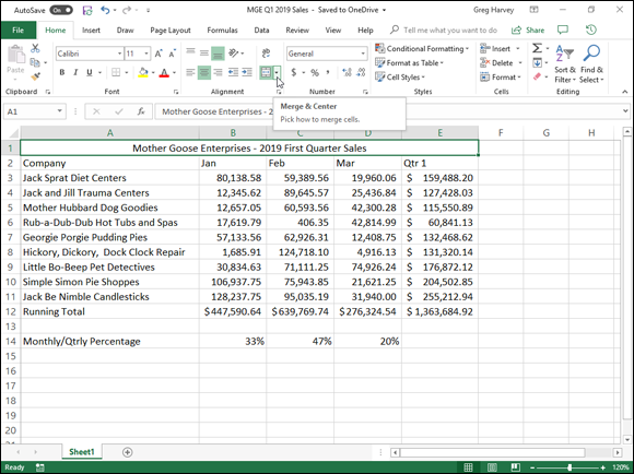
FIGURE 3-14: A worksheet title after merging and centering it across columns A through E.
If you ever need to split up a supercell that
you’ve merged with Merge & Center back into its original,
individual cells, select the cell and then simply click the Merge
& Center button in the Alignment group on the Home tab again.
You can also do this by clicking the drop-down button attached to
the Merge & Center button on the Home tab and then clicking
Unmerge Cells on this drop-down menu (a few more steps, I’d
say!).
Intent on indents
In Excel 2019, you can indent the entries in a cell selection by clicking the Increase Indent button. The Increase Indent button in the Alignment group of the Home tab sports a picture of an arrow pushing the lines of text to the right. Each time you click this button, Excel indents the entries in the current cell selection to the right by a little over a character width of the standard font. (See the section “Futzing with the Fonts,” earlier in this chapter, if you don’t know what a standard font is or how to change it.)
You can remove an indent by clicking the Decrease Indent button (to the immediate left of the Increase Indent button) on the Home tab with the picture of the arrow pushing the lines of text to the left. Additionally, you can change how many characters an entry indents with the Increase Indent button (or outdents with the Decrease Indent button). Open the Format Cells dialog box (Ctrl+1). Select the Alignment tab, and then alter the value in the Indent text box (by typing a new value in this text box or by dialing up a new value with its spinner buttons).
From top to bottom
Left, right, and center alignment all refer to the horizontal positioning of a text entry in relation to the left and right cell borders (that is, horizontally). You can also align entries in relation to the top and bottom borders of their cells (that is, vertically). Normally, all entries align vertically with the bottom of the cells (as though they were resting on the very bottom of the cell). You can also vertically center an entry in its cell or align it with the top of its cell.
To change the vertical alignment of a cell range that you’ve selected, click the appropriate button (Top Align, Middle Align, or Bottom Align) in the Alignment group on the Home tab.
Tampering with how the text wraps
Traditionally, column headings in worksheet tables have been a problem — you had to keep them really short or abbreviate them if you wanted to avoid widening all the columns more than the data warranted. You can avoid this problem in Excel by using the Wrap Text button in the Alignment group on the Home tab (the one to the immediate right of the Orientation button). In Figure 3-15, I show a new worksheet in which cells B2:H2 contain the names of various companies within the vast Mother Goose Enterprises conglomerate. Every company name that spills over to a column on the right that contains another name is truncated except for the Little Bo Peep Pet Detectives name in the last column in cell H2.

FIGURE 3-15: A new worksheet with truncated column headings in row 2.
Rather than widen columns B through H sufficiently to display the company names, I use the Wrap Text feature to avoid widening the columns as much as these long company names would otherwise require, as shown in Figure 3-16. To create the effect shown here, I select the cells with the column headings, B2:H2, and then click the Wrap Text button in the Alignment group on the Home tab.

FIGURE 3-16: Worksheet after using Wrap Text to display all the headings without widening their columns.
Selecting Wrap Text breaks up the long text entries (that either spill over or cut off) in the selection into separate lines. To accommodate more than one line in a cell, the program automatically expands the row height so that the entire wrapped-text entry is visible.
When you select Wrap Text, Excel continues to use the horizontal and vertical alignment you specify for the cell. You can use any of the Horizontal alignment options found on the Alignment tab of the Format Cells dialog box (Ctrl+1), including Left (Indent), Center, Right (Indent), Justify, or Center Across Selection. However, you can’t use the Fill option or Distributed (Indent) option. Select the Fill option on the Horizontal drop-down list box only when you want Excel to repeat the entry across the entire width of the cell.
If you want to wrap a text entry in its cell and have Excel justify the text with both the left and right borders of the cell, select the Justify option from the Horizontal drop-down list box in the Alignment tab in the Format Cells dialog box.
You can break a long text entry into separate
lines by positioning the insertion point in the cell entry (or on
the Formula bar) at the place where you want the new line to start
and pressing Alt+Enter. Excel expands the row containing the cell
(and the Formula bar above) when it starts a new line. When you
press Enter to complete the entry or edit, Excel automatically
wraps the text in the cell, according to the cell’s column width
and the position of the line break.
Reorienting cell entries
Instead of wrapping text entries in cells, you may find it more beneficial to change the orientation of the text by rotating the text up (in a counterclockwise direction) or down (in a clockwise direction). Peruse Figure 3-17 for a situation where changing the orientation of the wrapped column headings works much better than just wrapping them in their normal orientation in the cells.
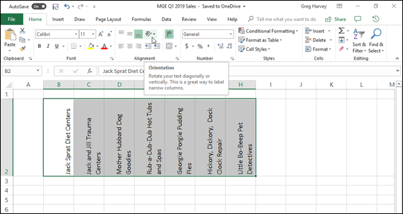
FIGURE 3-17: Column headings rotated 90° counterclockwise.
This example shows the same column headings for the sample order form I introduced in Figure 3-15 after rotating them 90 degrees counterclockwise. To make this switch with the cell range B2:H2 selected, click the Orientation button in the Alignment group on the Home tab and then click the Rotate Text Up option on the drop-down menu.
Figure 3-18 shows the same headings rotated up at a 45-degree angle. To create what you see in this figure, you click the Angle Counterclockwise option on the Orientation button’s drop-down menu after making the same cell selection, B2:H2.
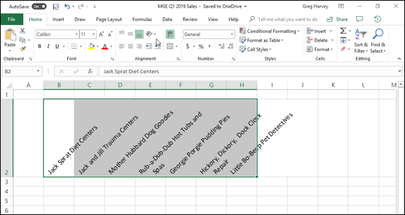
FIGURE 3-18: Column headings rotated 45° counterclockwise.
If you need to set the rotation of the entries in a spreadsheet at angles other than 45 and 90 degrees (up or down), you need to click the Format Cell Alignment option on the Orientation button’s drop-down menu. Doing so opens the Alignment tab of the Format Cells dialog box (or press Ctrl+1 and click the Alignment tab) where you can then use the controls in the Orientation section to set the angle and number of degrees.
To set a new angle, enter the number of degrees in the Degrees text box, click the appropriate place on the semicircular diagram, or drag the line extending from the word Text in the diagram to the desired angle.
To angle text up using the Degrees text
box, enter a positive number between 1 and 45 in the text box. To
angle the text down, enter a negative number between –1 and
–45.
To set the text vertically so that each letter is
above the other in a single column, select the Vertical Text option
on the Orientation button’s drop-down menu on the Home tab.
Shrink to fit
For those times when you need to prevent Excel from widening the column to fit its cell entries (as might be the case when you need to display an entire table of data on a single screen or printed page), use the Shrink to Fit text control.
Select the Alignment tab of the Format Cells dialog box (Ctrl+1) and then select the Shrink to Fit check box in the Text Control section. Excel reduces the font size of the entries to the selected cells so that they don’t require changing the current column width. Just be aware when using this Text Control option that, depending on the length of the entries and width of the column, you can end up with some text entries so small that they’re completely illegible!
Bring on the borders!
The gridlines you normally see in the worksheet to separate the columns and rows are just guidelines to help you keep your place as you build your spreadsheet. You can choose to print them with your data or not by checking or clearing the Print check box that appears in the Gridlines section of the Sheet Options group on the Ribbon’s Page Layout tab.
To emphasize sections of the worksheet or parts of a particular table, you can add borderlines or shading to certain cells. Don’t confuse the borderlines that you add to accent a particular cell selection with the gridlines used to define cell borders in the worksheet — borders that you add print regardless of whether you print the worksheet gridlines.
To see the borders that you add to the cells in a
worksheet, remove the gridlines normally displayed in the worksheet
by clearing the View check box in the Gridlines section of the
Sheet Options group on the Ribbon’s Page Layout tab.
To add borders to a cell selection, click the drop-down button attached to the Borders button in the Font group on the Home tab. This displays a drop-down menu with all the border options you can apply to the cell selection (see Figure 3-19) where you click the type of line you want to apply to all its cells.

FIGURE 3-19: Select borders for a cell selection on the Borders drop-down menu opened with the Borders button on the Home tab.
When selecting options on this drop-down menu to determine where you want the borderlines drawn, keep these things in mind:
- To have Excel draw borders only around the outside edges of the entire cell selection (in other words, following the path of the expanded cell cursor), click the Outside Borders or the Thick Box Border options on this menu. To draw the outside borders yourself around an unselected cell range in the active worksheet, click the Draw Border option, drag the mouse (using the Pencil mouse pointer) through the range of cells, and then click the Borders button on the Home tab’s Font group.
- If you want borderlines to appear around all four edges of each cell in the cell selection (like a paned window), select the All Borders option on this drop-down menu. If you want to draw the inside and outside borders yourself around an unselected cell range in the active worksheet, click the Draw Border Grid option, drag the mouse (using the Pencil mouse pointer) through the range of cells, and then click the Borders button on the Home tab.
To change the type of line, line thickness, or color of the borders you apply to a cell selection, you must open the Format Cells dialog box and use the options on its Border tab (click More Borders at the bottom of the Borders button’s drop-down menu or press Ctrl+1 and then click the Border tab).
To select a new line thickness or line style for a border you’re applying, click its example in the Style section. To change the color of the border you want to apply, click the color sample on the Color drop-down palette. After you select a new line style and/or color, apply the border to the cell selection by clicking the appropriate line in either the Presets or Border section of the Border tab before you click OK.
To get rid of existing borders in a
worksheet, you must select the cell or cells that presently contain
them and then click the No Border option at the top of the second
section on the Borders button’s drop-down menu.
Applying fill colors, patterns, and gradient effects to cells
You can also add emphasis to particular sections of the worksheet or one of its tables by changing the fill color of the cell selection and/or applying a pattern or gradient to it.
If you’re using a black-and-white printer, you
want to restrict your color choices to light gray in the color
palette. Additionally, you want to restrict your use of pattern
styles to the very open ones with few dots when enhancing a cell
selection that contains any kind of entries (otherwise, the entries
will be almost impossible to read when printed).
To choose a new fill color for the background of a cell selection, you can click the Fill Color button’s drop-down menu in the Font group on the Home tab and then select the color you want to use in the drop-down palette. Remember that you can use Live Preview to see what the cell selection looks like in a particular fill color by moving the mouse pointer over the color swatches. Click one to select it.
To choose a new pattern for a cell selection, you must open the Format Cells dialog box (Ctrl+1), and then click the Fill tab. To change the pattern of the cell selection, click a pattern swatch from the Pattern Style button’s pattern palette. To add a fill color to the pattern you select, click its color swatch in the Background Color section of the Fill tab.
If you want to add a gradient effect to the cell selection that goes from one color to another in a certain direction, click the Fill Effects button on the Fill tab to open the Fill Effects dialog box. This dialog box contains a Gradient tab with controls that enable you to determine the two colors to use as well as shading style and variant.
After you select the colors and styles of the gradient, check the Sample swatch in the Fill Effects dialog box. When you have it the way you want it, click OK to close the Fill Effects dialog box and return to the Format Cells dialog box. The selected gradient effect then appears in its Sample area on the Fill tab in the Format Cells dialog box. Unfortunately, this is one area where Live Preview doesn’t work, so you’re just going to have to click its OK button to apply the gradient to the cell selection to see how it actually looks in the worksheet.
Although you can’t select new patterns
or gradients (only colors) with the Fill Color button on the Home
tab, you can remove fill colors, patterns, and gradients assigned
to a cell selection by clicking the No Fill option on the Fill
Color button’s drop-down menu.
Doing It in Styles
In Excel 2019, vibrant cell styles are a snap to assign to your worksheet data using the Cell Styles gallery opened by selecting the Cell Styles button in the Styles group on the Ribbon’s Home tab. The Cell Styles gallery contains loads of ready-made styles you can immediately apply to the current cell selection. Simply click the desired style sample in the gallery after using the Live Preview feature to determine which style looks best on your data.
Creating a new style for the gallery
To create a new style for the gallery by example, manually format a single cell with all the attributes you want (font, font size, font color, bold, italic, underlining, fill color, pattern, borders, orientation, and so on) and then click the Cell Styles button on the Home tab followed by the New Cell Style option at the bottom of the gallery. Excel then opens a Style dialog box where you replace the generic style name (Style 1, Style 2, and so on) with your own descriptive name before you click OK.
Excel then adds a sample of your new style — the style name formatted, with the new style’s attributes — to a Custom section at the top of the Cell Styles gallery. To apply this custom style to a cell selection, you then only have to click its sample in the Custom section of the Cell Styles gallery.
The custom cell styles you create don’t
become part of the current workbook until the next time you save
the workbook. Therefore, you need to remember to click the Save
button on the Quick Access toolbar or press Ctrl+S to save your
changes after creating a new cell style if you want that style to
remain part of the workbook’s Cell Styles gallery the next time you
open the workbook in Excel.
Copying custom styles from one workbook into another
Excel makes it easy to copy custom cell styles that you’ve saved as part of one workbook into the workbook you’re currently working on. To copy custom styles from one workbook to another, follow these steps:
-
Open the workbook that needs the custom styles added to it from another existing workbook.
This can be a brand-new workbook or one that you’ve opened for editing (see Chapter 4).
-
Open the workbook that has the custom styles you want to copy saved as part of it.
See the previous section, “Creating a new style for the gallery,” for tips on how to create and save cell styles.
-
Switch back to the workbook into which you want to copy the saved custom styles.
You can do this by clicking the workbook’s button on the Windows taskbar or using the Flip feature by pressing Alt+Tab until you select the workbook’s thumbnail in the center of the display.
-
Click the Cell Styles button on the Home tab followed by Merge Styles in the Cell Styles gallery or press Alt+HJM.
Excel opens the Merge Styles dialog box.
- Click the name of the open workbook file that contains the custom styles to copy in the Merge Styles From list box and then click OK.
After you close the Merge Styles dialog box, Excel adds all the custom styles from the designated workbook into the current workbook, adding them to the Custom section of its Cell Styles gallery. To retain the custom styles you just imported, save the current workbook (click the Save button on the Quick Access toolbar or press Ctrl+S). Then, you can switch back to the workbook containing the original custom styles you just copied and close its file (press Alt+FC).
Fooling Around with the Format Painter
Using cell styles to format ranges of worksheet cells is certainly the way to go when you have to apply the same formatting repeatedly in the workbooks you create. However, there may be times when you simply want to reuse a particular cell format and apply it to particular groups of cells in a single workbook without ever bothering to open the Cell Styles gallery.
For those occasions when you feel the urge to format on the fly (so to speak), use the Format Painter button (the paintbrush icon) in the Clipboard group on the Home tab. This wonderful little tool enables you to take the formatting from a particular cell that you fancy up and apply its formatting to other cells in the worksheet simply by selecting those cells.
To use the Format Painter to copy a cell’s formatting to other worksheet cells, just follow these easy steps:
- Format an example cell or cell range in your workbook, selecting whatever fonts, alignment, borders, patterns, and color you want it to have.
-
Select one of the cells you just fancied up and click the Format Painter button in the Clipboard group on the Home tab.
The mouse pointer changes from the standard thick, white cross to a thick, white cross with an animated paintbrush by its side, and you see a marquee around the selected cell with the formatting to be used by the Format Painter.
-
Drag the white-cross-plus-animated-paintbrush pointer (the Format Painter pointer) through all the cells you want to format.
As soon as you release the mouse button, Excel applies all the formatting used in the example cell to all the cells you just selected!
To keep the Format Painter selected so that you can format a bunch of different cell ranges with the Format Painter pointer, double-click the Format Painter button on the Home tab after you select the sample cell with the desired formatting. To stop formatting cells with the Format Painter pointer, you simply click the Format Painter button on the Home tab again (it remains selected when you double-click it) to restore the button to its unselected state and return the mouse pointer to its normal thick, white cross shape.
You can use the
Format Painter to restore a cell range that you gussied all up back
to its boring default (General) cell format. To do this, click an
empty, previously unformatted cell in the worksheet before you
click the Format Painter button and then use the Format Painter
pointer to drag through the cells you want returned to the default
General format.
Using the Format Painter on a
touchscreen has a very limited application: You can only copy the
formatting from the one cell to another by first tapping the
formatted cell and then tapping the cell to be formatting.
Unfortunately, you can’t format an entire cell range by dragging
your finger or stylus as you can with the mouse.
Conditional Formatting
Before leaving behind the scintillating subject of cell formatting, there’s one more formatting button in the Styles group of the Home tab of which you need to be aware. The Conditional Formatting button enables you to apply provisional formatting to a cell range based solely on the categories into which its current values fall. The cool thing about this kind of conditional formatting is that should you edit the numbers in the cell range so that their values fall into other categories, the program automatically changes their cell formatting to suit.
When you click the Conditional Formatting button in the Styles group of the Home tab, a drop-down menu appears with the following options:
- Highlight Cells Rules opens a continuation menu with various options for defining formatting rules that highlight the cells in the cell selection that contain certain values, text, or dates; that have values greater or less than a particular value; or that fall within a certain ranges of values.
- Top/Bottom Rules opens a continuation menu with various options for defining formatting rules that highlight the top and bottom values, percentages, and above and below average values in the cell selection.
- Data Bars opens a palette with different color data bars that you can apply to the cell selection to indicate their values relative to each other by clicking the data bar thumbnail.
- Color Scales opens a palette with different two- and three-colored scales that you can apply to the cell selection to indicate their values relative to each other by clicking the color scale thumbnail.
- Icon Sets opens a palette with different sets of icons that you can apply to the cell selection to indicate their values relative to each other by clicking the icon set.
- New Rule opens the New Formatting Rule dialog box where you define a custom conditional formatting rule to apply to the cell selection.
- Clear Rules opens a continuation menu where you can remove conditional formatting rules for the cell selection by clicking the Clear Rules from Selected Cells option, for the entire worksheet by clicking the Clear Rules from Entire Sheet option, or for just the current data table by clicking the Clear Rules from This Table option. If you’re working with a Pivot Table (as described in Chapter 9), you can clear the conditional formatting from it by clicking the Clear Rules from This PivotTable option at the very bottom of this menu.
- Manage Rules opens the Conditional Formatting Rules Manager dialog box where you edit and delete particular rules as well as adjust their rule precedence by moving them up or down in the Rules list box.
Formatting with scales and markers
The easiest conditional formatting that you can apply to a worksheet cell range is using the pop-up palettes of graphical scales and markers attached to the Data Bars, Color Scales, and Icon Sets options on the Conditional Formatting button’s drop-down menu:
- Data Bars represent the relative values in the cell selection by the length of the color bar in each cell and are great for helping you quickly spot the lower and higher values within a large range of data.
- Color Scales classify the relative values in a cell selection with a color gradation using a one-, two-, or three-color scale and are great for identifying the distribution of values across a large range of data.
- Icon Sets classify the values in the cell selection into particular graphic sets arranged in four categories, and each icon within a set represents a range of values that go from high to low. Icon sets are great for quickly identifying the different ranges of values in a range of data.
Figure 3-20 shows you an example of cell ranges (containing identical values) using each of the three formatting types. The values in the first range (B2:B12) are conditionally formatted using blue Gradient Fill Data Bars. The values in the second range (D2:D12) are conditionally formatted using the Green, Yellow, Red Color Scale. The values in the third range (F2:F12) are conditionally formatted using the 3 Arrows (Colored) Icon Set.
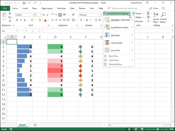
FIGURE 3-20: Sample worksheet with three identical cell ranges formatted with Excel’s Data Bars, Color Scales, and Icon Sets options.
In Figure 3-20, the particular conditional formatting types Excel assigned to each cell range can be interpreted as follows:
- Data bars added to the cells in the first cell range, B2:B12, represent the relative size of its values graphically, much like a standard bar chart.
- Color scales applied to the second range, D2:D12, represent the relative size of the values in the range by color and hue (red hues applied to the lower values, yellow to the middle values, and green to the higher values).
- Directional icons applied to the third cell range, F2:F12, represent the relative size of the values in the range with arrow icons pointing in different directions (arrows pointing straight down for the lower values, straight up for the higher values, and sideways for middling values).
Highlighting cells ranges
The Highlight Cells Rules and Top/Bottom Rules options on Excel’s Conditional Formatting drop-down menu enable you to quickly identify cell entries of particular interest in various cell ranges in your worksheet.
The options on the Highlight Cells Rules continuation menu enable you to set formats that identify values that are greater than, less than, equal to, or even between particular values that you set. This menu also contains an option for setting special formats for identifying cells that contain particular text (such as Yes, No, or even Maybe answers in a data list) or certain dates (such as project milestones and deadlines).
Perhaps one of the most useful options on the
Highlight Cells Rules continuation menu is the Duplicate Values
option that enables you to flag duplicate entries in a cell range
by assigning them a special formatting. Doing this not only makes
it easy to visually identify duplicate entries in a data list or
table but also to find them electronically by searching for their
particular formatting characteristics. (See Chapter 6 for details on searching your
worksheets.)
The options on the Top/Bottom Rules continuation menu enable you to specially format and, therefore, easily identify values in data tables and lists that are either above or below the norm. These options not only include those for automatically formatting all values in a range that are among the top 10 highest or lowest (either in value or percentage) but also above or below the average (as calculated by dividing the total by the number of values).
In addition to using the ready-made
rules for conditional formatting located on the Highlight Cells
Rules and Top/Bottom Rules continuation menus, you can also create
your own custom rules. When you create a custom rule, you not only
specify the rule type that identifies which values or text entries
to format, but also you format the colors and other aspects
included in the formatting. (For details on creating custom
conditional formats, consult my Excel 2019 All-in-One For
Dummies.)
Formatting via the Quick Analysis tool
One of the quickest and easiest ways to apply Data Bars, Color Scales, Icon Set, Greater Than, or Top 10% conditional formatting to a data table is with the Excel 2019’s Quick Analysis tool. The coolest thing about applying conditional formatting in this manner is that Live Preview lets you visualize how your data looks with a particular type of conditional formatting before you actually apply it.
To assign conditional formatting with the Quick Analysis tool, select the data in your table that you wanted formatted and then select the Quick Analysis tool. By default, the Formatting option is selected when Excel displays the tool’s palette so that all you have to do is highlight each of the formatting options with your mouse or Touch pointer to see how they will look on your data.
Figure 3-21 shows you the Live Preview of the financial data in the Mother Goose 2016 Sales table with the Data Bars conditional formatting (as the Data Bars button is highlighted in the Formatting options). To assign this conditional format to the financial data in the selected table, you simply click the Data Bars button on the Quick Analysis palette. To preview how the data would look formatted with another conditional format, you simply highlight its button with the mouse or Touch pointer.
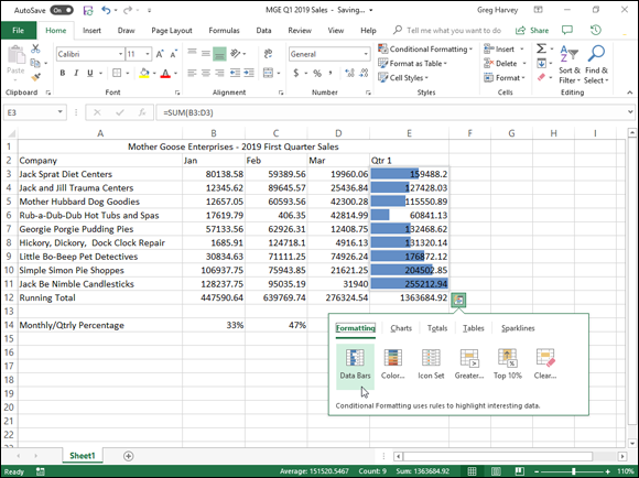
FIGURE 3-21: Previewing conditional formatting in a data table using the Quick Analysis tool.
Note that if you click the Greater Than button on the Quick Analysis palette, Excel displays a Greater Than dialog box where you specify the threshold value in the Format Cells That Are Greater Than text box, as well as select the color of the formatting for all the cells above that threshold in the drop-down list to its right.
With all the other kinds of conditional formats (Data Bars, Color Scales, Icon Set, and Top 10%), Excel just goes ahead and applies the first (default) option for that kind of formatting that you find on the Conditional Formatting button’s drop-down menus on the Ribbon.