Prev Next

S. Suzanne NielsenFood Analysis Laboratory ManualFood Science Text Serieshttps://doi.org/10.1007/978-3-319-44127-6_2

2. Preparation of Reagents and Buffers

Catrin Tyl¹ and Baraem P. Ismail¹

(1)

Department of Food Science and Nutrition, University of Minnesota, St. Paul, MN, USA

Catrin Tyl (Corresponding author)

Email: Tylxx001@umn.edu

Baraem P. Ismail

Email: bismailm@umn.edu

2.1 Preparation of Reagents of Specified Concentrations

Virtually every analytical method involving wet chemistry starts with preparing reagent solutions. This usually involves dissolving solids in a liquid or diluting from stock solutions. The concentration of analytes in solution can be expressed in weight (kg, g, or lower submultiples) or in the amount of substance (mol), per a unit volume (interchangeably L or dm³, mL or cm³, and lower submultiples). Preparing reagents of correct concentrations is crucial for the validity and reproducibility of any analytical method. Below is a sample calculation to prepare a calcium chloride reagent of a particular concentration.

Example A1

How much calcium chloride do you need to weigh out to get 2 L of a 4 mM solution?

Solution

The molarity (M) equals the number of moles (n) in the volume (v) of 1 L:

$M\left(\frac{\mathrm{mol}}{\mathrm{L}}\right) = \frac{n\ \left(\mathrm{mol}\right)}{v\left[\mathrm{L}\right]}$

(2.1)

The desired molarity is 4 mM = 0.004 M; the desired volume is 2 L. Rearrange Eq. 2.1 so that:

$n\ \left(\mathrm{mol}\right) = M\left(\frac{\mathrm{mol}}{\mathrm{L}}\right) \times v\ \left(\mathrm{L}\right)$

(2.2)

The mass (m) of 1 mole CaCl₂ (110.98 g/mol) is specified by the molecular weight (MW) as defined through Eq. 2.3. The mass to be weighed is calculated by rearranging into Eq. 2.4:

$\mathrm{MW}\ \left(\frac{\mathrm{g}}{\mathrm{mol}}\right) = \frac{m\ \left(\mathrm{g}\right)}{n\ \left(\mathrm{mol}\right)}$

(2.3)

$m\ \left(\mathrm{g}\right) = n\ \left(\mathrm{mol}\right) \times \mathrm{MW}\ \left(\frac{\mathrm{g}}{\mathrm{mol}}\right)$

(2.4)

Now substitute Eq. 2.2 into Eq. 2.4. Some of the units then cancel out, indicated as strike-throughs:

$m\ \left(\mathrm{g}\right) = M\ \left(\frac{\mathrm{mol}}{\mathrm{L}}\right) \times v\ \left(\mathrm{L}\right) \times \mathrm{MW}\ \left(\frac{\mathrm{g}}{\mathrm{mol}}\right)$

(2.5)

/epubstore/N/S-S-Nielsen/Food-Analysis-Laboratory-Manual/OEBPS/images/104615_3_En_2_Chapter/104615_3_En_2_Equ6_HTML.png

(2.6)

Example A2

How much would you need to weigh out if you were using the dihydrate (i.e., CaCl₂ ^.2H₂O) to prepare 2 L of a 4 mM solution of calcium chloride?

Solution

During crystallization of salts, water may be incorporated into the crystal lattice. Examples include phosphate salts, calcium chloride, and certain sugars. The names of these compounds are amended by the number of bound water molecules. For example, Na₂HPO₄ ^.7H₂O is called sodium monophosphate heptahydrate, and CaCl₂ ^.2H₂O is called calcium chloride dihydrate. The water is tightly bound and is not visible (the dry reagents do not look clumped). Many commercially available salts are sold as hydrates that can be used analogously to their dry counterparts after adjusting for their increased molecular weight, which includes the bound water molecules. The molecular weight of CaCl₂ changes from 110.98 g/mol to 147.01 g/mol to account for two molecules of water at about 18 g/mol. Hence, Eq. 2.6 needs to be modified to:

/epubstore/N/S-S-Nielsen/Food-Analysis-Laboratory-Manual/OEBPS/images/104615_3_En_2_Chapter/104615_3_En_2_Equ7_HTML.png

(2.7)

Thus, 1.176 g of CaCl₂ would be weighed out and the volume made up to 2 L in a volumetric flask.

Other commonly used ways to express concentrations are listed in Table 2.1. For instance, for very low concentrations as encountered in residue analysis, parts per million (e.g., μg/mL or mg/L) and parts per billion (e.g., μg/L) are preferred units. Concentrated acids and bases are often labeled in percent mass by mass or percent mass per volume. For instance, a 28 % wt/wt solution of ammonia in water contains 280 g ammonia per 1000 g of solution. On the other hand, 32 % wt/vol NaOH solution contains 320 g of NaOH per L. For dilute solutions in water, the density is approximately 1 kg/L at room temperature (the density of water is exactly 1 kg/L only at 5 °C), and thus wt/wt and wt/vol are almost equal. However, concentrated solutions or solutions in organic solvents can deviate substantially in their density. Therefore, for concentrated reagents, the correct amount of reagent needed for dilute solutions is found by accounting for the density, as illustrated in Example A3 below:

table 2.1

Concentration expression terms

Unit	Symbol	Definition	Relationship
Molarity	M	Number of moles of solute per liter of solution	$\mathrm{M}\kern0.5em =\kern0.5em \frac{\mathrm{mol}}{\mathrm{liter}}$
Normality	N	Number of equivalents of solute per liter of solution	$\mathrm{N}\kern0.5em =\kern0.5em \frac{\mathrm{equivalents}}{\mathrm{liter}}$
Percent by weight (parts per hundred)	wt %	Ratio of weight of solute to weight of solute plus weight of solvent × 100	$\mathrm{wt}\ \%\kern0.5em =\kern0.5em \frac{\mathrm{wt}\kern0.5em \mathrm{solute}\kern0.5em \times \kern0.5em 100}{\mathrm{total}\kern0.5em \mathrm{wt}}$
	wt/vol %	Ratio of weight of solute to total volume × 100	$\mathrm{wt}/\mathrm{vol}\ \%\kern0.5em =\kern0.5em \frac{\mathrm{wt}\kern0.5em \mathrm{solute}\kern0.5em \times \kern0.5em 100}{\mathrm{total}\kern0.5em \mathrm{volume}}$
Percent by volume	vol %	Ratio of volume of solute to total volume × 100	$\mathrm{vol}\kern0.5em \%\kern0.5em =\kern0.5em \frac{\mathrm{vol}\kern0.5em \mathrm{of}\kern0.5em \mathrm{solute}\kern0.5em \times \kern0.5em 100}{\mathrm{total}\kern0.5em \mathrm{volume}}$
Parts per million	ppm	Ratio of solute (wt or vol) to total weight or volume × 1,000,000	$\mathrm{ppm}\kern0.5em =\kern0.5em \frac{\mathrm{mg}\kern0.5em \mathrm{solute}}{\mathrm{kg}\kern0.5em \mathrm{solution}}$ $=\kern0.5em \frac{\mu \mathrm{g}\kern0.5em \mathrm{solute}}{\mathrm{g}\kern0.5em \mathrm{solution}}$ $=\kern0.5em \frac{\mathrm{mg}\kern0.5em \mathrm{solute}}{\mathrm{L}\kern0.5em \mathrm{solution}}$ $=\kern0.5em \frac{\mu \mathrm{g}\kern0.5em \mathrm{solute}}{\mathrm{mL}\kern0.5em \mathrm{solution}}$
Parts per billion	ppb	Ratio of solute (wt or vol) to total weight or volume × 1,000,000,000	$\mathrm{ppb}\kern0.5em =\kern0.5em \frac{\mu \mathrm{g}\kern0.5em \mathrm{solute}}{\mathrm{kg}\kern0.5em \mathrm{solution}}$ $=\kern0.5em \frac{\mathrm{ng}\kern0.5em \mathrm{solute}}{\mathrm{g}\kern0.5em \mathrm{solution}}$ $=\kern0.5em \frac{\mu \mathrm{g}\kern0.5em \mathrm{solute}}{\mathrm{L}\kern0.5em \mathrm{solution}}$ $=\kern0.5em \frac{\mathrm{ng}\kern0.5em \mathrm{solute}}{\mathrm{mL}\kern0.5em \mathrm{solution}}$

Example A3

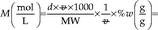
Prepare 500 mL of a 6 M sulfuric acid solution from concentrated sulfuric acid. The molecular weight is 98.08 g/mol, and the manufacturer states that it is 98 % wt/wt and has a density (d) of 1.84 g/mL.

Solution

The density specifies the mass per volume of the concentrated H₂SO₄:

$d = \frac{m}{v}\ \left(\frac{\mathrm{g}}{m\mathrm{L}}\right)$

(2.8)

The molarity of the concentrated sulfuric acid is determined by rearranging Eqs. 2.3 and 2.8 to express the unknown number of moles (n) in terms of known quantities (MW and d). However, because molarity is specified in moles per L, the density needs to be multiplied by 1000 to obtain the g per L (the unit of density is g per mL or kg per L).

$\mathrm{Rearrange}\kern0.5em \mathrm{Eq}.\ 3:\kern0.5em n\ \left(\mathrm{mol}\right) = \frac{m\ \left(\mathrm{g}\right)}{\mathrm{MW}\ \left(\frac{\mathrm{g}}{\mathrm{mol}}\right)\ }$

(2.9)

$\mathrm{Rearrange}\ \mathrm{Eq}.\ 8:\ m\ \left(\mathrm{g}\right) = d\ \left(\frac{\mathrm{g}}{\mathrm{L}}\right)\times 1000 \times v\ \left(\mathrm{L}\right)$

(2.10)

$\begin{array}{l}\mathrm{Substitute}\kern0.5em \mathrm{Eq}.\ 10\kern0.5em \mathrm{into}\kern0.5em \mathrm{Eq}.\ 9:\ \\ {}\kern5em n\ \left(\mathrm{mol}\right) = \kern0.5em \frac{d \times 1000\ \left(\frac{\mathrm{g}}{\mathrm{L}}\right) \times v\ \left(\mathrm{L}\right)}{\mathrm{MW}\ \left(\ \frac{\mathrm{mol}}{\mathrm{g}}\right)}\end{array}$

(2.11)

Substitute Eq. 2.11 into Eq. 2.1. The 98 % wt/wt (see Table 2.1) can be treated like a proportionality factor: every g of solution contains 0.98 g H₂SO₄. To account for this, multiply Eq. 2.1 with the wt %:

/epubstore/N/S-S-Nielsen/Food-Analysis-Laboratory-Manual/OEBPS/images/104615_3_En_2_Chapter/104615_3_En_2_Equ12_HTML.png

(2.12)

$M\ \left(\frac{\mathrm{mol}}{\mathrm{L}}\right) = \frac{d \times 1000\left(\frac{\mathrm{g}}{\mathrm{L}}\right)}{\mathrm{MW}\ \left(\frac{\mathrm{g}}{\mathrm{mol}}\right)} \times \% w\ \left(\frac{\mathrm{g}}{\mathrm{g}}\right)$

(2.13)

/epubstore/N/S-S-Nielsen/Food-Analysis-Laboratory-Manual/OEBPS/images/104615_3_En_2_Chapter/104615_3_En_2_Equ14_HTML.png

(2.14)

The necessary volume to supply the desired amount of moles for 500 mL of a 6 M solution is found by using Eq. 2.15:

${v}_1\left(\mathrm{L}\right) \times {M}_1\left(\frac{\mathrm{mol}}{\mathrm{L}}\right) = {v}_2\left(\mathrm{L}\right) \times {M}_2\left(\frac{\mathrm{mol}}{\mathrm{L}}\right)$

(2.15)

/epubstore/N/S-S-Nielsen/Food-Analysis-Laboratory-Manual/OEBPS/images/104615_3_En_2_Chapter/104615_3_En_2_Equ16_HTML.png

(2.16)

$\begin{array}{c} v\ \left(\mathrm{L}\right) = \frac{0.5\ \left(\mathrm{L}\right) \times 6\ }{18.39\ }\ \\ {}=0.163\ \mathrm{L}\kern0.5em \mathrm{or}\kern0.5em 163\ \mathrm{mL}\end{array}$

(2.17)

Hence, to obtain 500 mL, 163 mL concentrated sulfuric acid would be combined with 337 mL of water (500–163 mL). The dissolution of concentrated sulfuric acid in water is an exothermic process, which may cause splattering, and glassware can get very hot (most plastic containers are not suited for this purpose!). The recommended procedure would be to add some water to a 500 mL volumetric glass flask, e.g., ca. 250 mL, then add the concentrated acid, allow the mixture to cool down, mix, and bring up to volume with water.

2.2 Use of Titration to Determine Concentration of Analytes

A wide range of standard methods in food analysis, such as the iodine value, peroxide value and titratable acidity, involve the following concept:

A reagent of known concentration (i.e., the titrant)is titrated into a solution of analyte with unknown concentration. The used up volume of the reagent solution is measured.
The ensuing reaction converts the reagent and analyte into products.
When all of the analyte is used up, there is a measurable change in the system, e.g., in color or pH.
The concentration of the titrant is known; thus the amount of converted reactant can be calculated. The stoichiometry of the reaction allows for the calculation of the concentration of the analyte, for example, in the case of iodine values, the absorbed grams of iodine per 100 g of sample; in the case of peroxide value, milliequivalents of peroxide per kg of sample; or in the case of titratable acidity, % wt/vol acidity.

There are two principle types of reactions for which this concept is in widespread use: acid-base and redox reactions. For both reaction types, the concept of normality (N) plays a role, which signifies the number of equivalents of solute per L of solution. The number of equivalents corresponds to the number of transferred H⁺ for acid-base reactions and transferred electrons for redox reactions. Normality equals the product of the molarity with the number of equivalents (typically 1–3 for common acids and bases with low molecular weight), i.e., it is equal to or higher than the molarity. For instance, a 0.1 M sulfuric acid solution would be 0.2 N, because two H⁺ are donated per molecule H₂SO₄. On the other hand, a 0.1 M NaOH solution would still be 0.1 N, as indicated by Eq. 2.18:

$\mathrm{Normality} = \mathrm{Molarity}\times \mathrm{number}\ \mathrm{of}\ \mathrm{equivalents}$

(2.18)

Substituting N for M, reaction equivalence can be expressed through a modified version of Eq. 2.15 (which is the same as Refr. [4], Sect. 22.2.2, Eq. 2.1):

$\begin{array}{c} v\kern0.5em \mathrm{of}\ \mathrm{titrant}\kern0.5em \times N\ \mathrm{of}\ \mathrm{titrant} = \kern0.5em v\kern0.5em \mathrm{of}\kern0.5em \mathrm{analyte}\kern0.5em \mathrm{solution}\ \\ {}\times \kern0.5em N\kern0.5em \mathrm{of}\kern0.5em \mathrm{analyte}\kern0.5em \mathrm{solution}\end{array}$

(2.19)

Some analyses (such as in titratable acidity) require the use of equivalent weights instead of molecular weights. These can be obtained by dividing the molecular weight by the number of equivalents transferred over the course of the reaction.

/epubstore/N/S-S-Nielsen/Food-Analysis-Laboratory-Manual/OEBPS/images/104615_3_En_2_Chapter/104615_3_En_2_Equ20_HTML.png

(2.20)

Using equivalent weights can facilitate calculations, because it accounts for the number of reactive groups of an analyte. For H₂SO₄, the equivalent weight would be $\frac{98.08}{2}$ = 49.04 g/mol, whereas for NaOH it would be equal to the molecular weight since there is only one OH group.

To illustrate the concept, the reaction of acetic acid with sodium hydroxide in aqueous solution is stated below:

${\mathrm{CH}}_3\mathrm{COOH}+\mathrm{NaOH}\to {\mathrm{CH}}_3{\mathrm{COO}}^{-}+{\mathrm{H}}_2\mathrm{O}+{\mathrm{Na}}^{+}$

This reaction can form the basis for quantifying acetic acid contents in vinegar (for which it is the major acid):

Example B1

100 mL of vinegar is titrated with a solution of NaOH that is exactly 1 M. (Chapter 21, Sect. 21.2, in this laboratory manual describes how to standardize titrants.) If 18 mL of NaOH are used up, what is the corresponding acetic acid concentration in vinegar?

Solution

The reaction equation shows that both NaOH and CH₃COOH have an equivalence number of 1, because they each have only one reactive group. Thus, their normality and molarity are equal. Equation 2.19 can be used to solve Example B1, and the resulting N will, in this case, equal the M:

$\begin{array}{l}18\ \left(\mathrm{mL}\right)\kern0.5em \times \kern0.5em 1\left(\frac{\mathrm{mol}}{\mathrm{L}}\right)\kern0.5em =\kern0.5em 100\ \left(\mathrm{mL}\right)\kern0.5em \times \kern0.5em \mathrm{Normality}\ \\ {}\kern4.25em \mathrm{of}\kern0.5em \mathrm{acetic}\kern0.5em \mathrm{acid}\kern0.5em \mathrm{solution}\kern0.5em \left(\frac{\mathrm{mol}}{\mathrm{L}}\right)\end{array}$

(2.21)

/epubstore/N/S-S-Nielsen/Food-Analysis-Laboratory-Manual/OEBPS/images/104615_3_En_2_Chapter/104615_3_En_2_Equ22_HTML.png

(2.22)

Sometimes the stoichiometry of a reaction is different, such as when NaOH reacts with malic acid, the main acid found in apples and other fruits.

/epubstore/N/S-S-Nielsen/Food-Analysis-Laboratory-Manual/OEBPS/images/104615_3_En_2_Chapter/104615_3_En_2_Figa_HTML.png

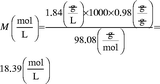
Example B2

Assume that 100 mL of apple juice are titrated with 1 M NaOH, and the volume used is 36 mL. What is the molarity of malic acid in the apple juice?

Solution

Malic acid contains two carboxylic groups, and thus for every mole of malic acid, two moles of NaOH are needed to fully ionize it. Therefore, the normality of malic acid is two times the molarity. Again, use Eq. 2.19 to solve Example B2:

$\begin{array}{l}36\ \left(\mathrm{mL}\right)\kern0.5em \times \kern0.5em 1\left(\frac{\mathrm{mol}}{\mathrm{L}}\right)\kern0.5em =\kern0.5em 100\ \left(\mathrm{mL}\right)\kern0.5em \times \kern0.5em 2\kern0.5em \\ {}\kern5em \times M\kern0.5em \mathrm{of}\kern0.5em \mathrm{malic}\ \mathrm{acid}\ \mathrm{solution}\kern0.5em \left(\frac{\mathrm{mol}}{\mathrm{L}}\right)\kern0.5em \end{array}$

(2.23)

/epubstore/N/S-S-Nielsen/Food-Analysis-Laboratory-Manual/OEBPS/images/104615_3_En_2_Chapter/104615_3_En_2_Equ24_HTML.png

(2.24)

This is the same value as obtained above for acetic acid. However, as a direct consequence of malic acid having two carboxyl groups instead of one, twice the amount of NaOH was needed.

Tables, calculators, and other tools for calculating molarities, normalities, and % acidity are available in print and online literature. However, it is important for a scientist to know the stoichiometry of the reactions involved, and the reactivity of reaction partners to correctly interpret these tables.

The concept of normality also applies to redox reactions; only electrons instead of protons are transferred. For instance, potassium dichromate, K₂Cr₂O₇, can supply six electrons, and therefore the normality of a solution would be six times its molarity. While the use of the term normality is not encouraged by the IUPAC, the concept is ubiquitous in food analysis because it can simplify and speed up calculations.

For a practical application of how normality is used to calculate results of titration experiments, see Chap. 21 in this laboratory manual.

2.3 Preparation of Buffers

A buffer is an aqueous solution containing comparable molar amounts of either a weak acid and its corresponding base or a weak base and its corresponding acid. A buffer is used to keep a pH constant. In food analysis, buffers are commonly used in methods that utilize enzymes, but they also arise whenever weak acids or bases are titrated. To explain how a weak acid or base and its charged counterpart manage to maintain a certain pH, the “comparable molar amounts” part of the definition is key: For a buffer to be effective, its components must be present in a certain molar ratio. This section is intended to provide guidance on how to solve calculation and preparation problems relating to buffers. While it is important for food scientists to master calculations of buffers, the initial focus will be on developing an understanding of the chemistry. Figures 2.1 and 2.2 show an exemplary buffer system, and how the introduction of strong acid would affect it.

/epubstore/N/S-S-Nielsen/Food-Analysis-Laboratory-Manual/OEBPS/images/104615_3_En_2_Chapter/104615_3_En_2_Fig1_HTML.png — figure 2.1
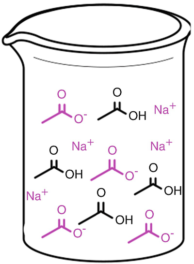
A buffer solution composed of the weak acetic acid, CH₃COOH, and a salt of its corresponding base, sodium acetate, CH₃COO⁻Na⁺. In aqueous solution, the sodium acetate dissociates into CH₃COO⁻ (acetate ions) and Na⁺ (sodium ions), and for this reason, these ions are drawn spatially separated. The Na⁺ ions do not participate in buffering actions and can be ignored for future considerations. Note that the ratio of acetic acid and acetate is equal in our example. Typical buffer systems have concentrations between 1 and 100 mM

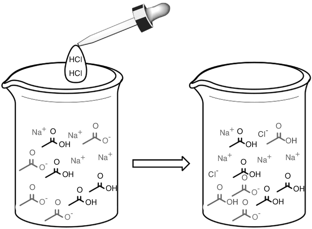
/epubstore/N/S-S-Nielsen/Food-Analysis-Laboratory-Manual/OEBPS/images/104615_3_En_2_Chapter/104615_3_En_2_Fig2_HTML.png — figure 2.2
Changes induced by addition of the strong acid HCl, to the buffer from Fig. 2.1. HCl can be considered as completely dissociated into Cl⁻ and H⁺. The H⁺ combines with CH₃COO⁻ instead of H₂O, because CH₃COO⁻ is the stronger base. Thus, instead of H₃O⁺, additional CH₃COOH is formed. This alters the ratio between CH₃COOH and CH₃COO⁻, resulting in a different pH as illustrated in problem C2. The Cl⁻ ions are merely counterions to balance charges but do not participate in buffer reactions and can thus be ignored

Only weak acids and bases can form buffers. The distinction of strong versus weak acids/bases is made based on how much of either H₃O⁺ or OH⁻ is generated, respectively. Most acids found in foods are weak acids; hence, once the equilibrium has been reached, only trace amounts have dissociated, and the vast majority of the acid is in its initial, undissociated state. For the purpose of this discussion, we will refer to the buffer components as acid AH, undissociated state, and corresponding base A ⁻, concentrations can be measured and are published in the form of dissociation constants, K _a , or their negative logarithms to base 10, pK _a values. These values can be found on websites of reagent manufacturers as well as numerous other websites and textbooks. Table 2.2 lists the pK_a values of some common acids either present in foods or often used to prepare buffers, together with the acid’s molecular and equivalent weights. However, reported literature values for K_a/pK_a can be different for the same compound. For instance, they range between 6.71 and 7.21 for H₂PO₄ ⁻. Dissociation constants depend on the ionic strength of the system, which is influenced by the concentrations of all ions in the system, even if they do not buffer. In addition, the pH in a buffer system is, strictly speaking, determined by activities, not by concentrations (see Refr. [4], Sect. 22.3.2.1). However, for concentrations <0.1 M, activities are approximately equal to concentrations, especially for monovalent ions. For H₂PO₄ ⁻, the value 7.21 is better suited for very dilute systems. For buffers intended for media or cell culture, the system typically contains several salt components, and 6.8 would be a commonly used value. If literature specifies several pK_a values, try finding information on the ionic strength where these values were obtained and calculate/estimate the ionic strength of the solution where the buffer is to be used. However, even for the same ionic strength, there may be different published values, depending on the analytical method. When preparing a buffer (see notes below), always test and, if necessary, adjust the pH, even for commercially available dry buffer mixes that only need to be dissolved. The values listed in Table 2.2 are for temperatures of 25 °C and ionic strengths of 0 M, as well as 0.1 M, if available.

table 2.2

Properties of common food acids

	Formula	pK_a1	pK_a2	pK_a3	Molecular weight	Equivalent weight
Acetic acid	CH₃COOH	4.75^b	–	–	60.06	60.06
Carbonic acid	H₂CO₃	6.4^b	10.3^b	–	62.03	31.02
Carbonic acid	H₂CO₃	6.1^c	9.9^c	–	62.03	31.02
Citric acid	HOOCCH₂C(COOH)OHCH₂COOH	3.13^b	4.76^b	6.40^b	192.12	64.04
Citric acid	HOOCCH₂C(COOH)OHCH₂COOH	2.90^c	4.35^c	5.70^c	192.12	64.04
Formic acid	HCOOH	3.75^b	–	–	46.03	46.03
Lactic acid	CH₃CH(OH)COOH	3.86	–	–	90.08	90.08
Malic acid	HOOCCH₂CHOHCOOH	3.5^b	5.05^b	–	134.09	67.05
Malic acid	HOOCCH₂CHOHCOOH	3.24^c	4.68^c
Oxalic acid	HOOCCOOH	1.25^b	4.27^b	–	90.94	45.02
Oxalic acid	HOOCCOOH	1.2^c	3.80^c	–	90.94	45.02
Phosphoric acid	H₃PO₄	2.15^b	7.20^b	12.38^b	98.00	32.67
Phosphoric acid	H₃PO₄	1.92^c	6.71^c	11.52^c	98.00	32.67
Potassium acid phthalate	HOOCC₆H₄COO⁻K⁺	5.41^b	–	–	204.22	204.22
Tartaric acid^a	HOOCCH(OH)CH(OH)COOH	3.03	4.45	–	150.09	75.05

Data from Refs. [1, 2]

^aDissociation constants depend on the stereoisomer (D/L vs. meso-form). Values given for the naturally occurring R,R enantiomer (L-form)

^bAt ionic strength of 0 M

^cAt ionic strength of 0.1 M

Maximum buffering capacity always occurs around the pK_a value of the acid component. At the pK_a, the ratio of acid/corresponding base is 1:1 (not, as often erroneously assumed, 100:0). Therefore, a certain acid/corresponding base pair is suitable for buffering a pH range of pK_a ± 1. The molarity of a buffer refers to the sum of concentration for acid and corresponding base. The resulting pH of a buffer is governed by their concentration ratio, as described through the Henderson-Hasselbalch equation:

$\mathrm{pH} = {\mathrm{pK}}_{\mathrm{a}} + \log\ \frac{\left[{\mathrm{A}}^{-}\right]}{\left[\mathrm{AH}\right]}$

(2.25)

Weak bases such as ammonia, NH₃, can also form buffers with their corresponding base, in this case NH₄ ⁺. The Henderson-Hasselbalch equation would actually not change, since NH₄ ⁺ would serve as the acid, denoted BH, and the base NH₃ is denoted as B. The acid component is always the form with more H⁺ to donate. However, you may find the alternative equation:

$\mathrm{pOH} = {\mathrm{pK}}_{\mathrm{b}} + \log\ \frac{\left[{\mathrm{BH}}^{+}\right]}{\left[\mathrm{B}\right]}$

(2.26)

The pH would then be calculated as 14 − pOH. The term pOH refers to the concentration of OH⁻, which increases when bases are present in the system (see Ref. [4], Sect. 22.3, for details). However, using Eq. 2.25 and BH⁺ instead of AH as well as B in place of A⁻ gives the same result, as the pK_b is related to the pK_a through 14 − pK_b = pK_a.

Below are several examples of buffer preparation using the Henderson-Hasselbalch equation:

Example C1

What is the pH of a buffer obtained by mixing 36 mL of a 0.2 M Na₂HPO₄ solution and 14 mL of a 0.2 M NaH₂PO₄ solution, after adding water to bringing the volume to 100 mL to obtain a 0.1 M buffer?

Solution

The Henderson-Hasselbalch equation requires knowledge of the acidic component’s pK_a value and the concentrations of both buffer components. Rearrange Eq. 2.15 so that:

$\begin{array}{l} M\ \mathrm{in}\ \mathrm{buffer}\ \left(\frac{\mathrm{mol}}{\mathrm{L}}\right) = \\ {}\kern3.75em \frac{\begin{array}{l}\kern1em \\ {}\begin{array}{c} M\ \mathrm{of}\ \mathrm{stock}\\ {}\mathrm{solutions}\ \left(\frac{\mathrm{mol}}{\mathrm{L}}\right) \times \begin{array}{c} v\ \mathrm{of}\ \mathrm{stock}\\ {}\mathrm{solutions}\ \left(\frac{\mathrm{mol}}{\mathrm{L}}\right)\ \end{array}\end{array}\end{array}}{\ v\ \mathrm{of}\ \mathrm{buffer}\ \left(\mathrm{L}\right)}\end{array}$

(2.27)

/epubstore/N/S-S-Nielsen/Food-Analysis-Laboratory-Manual/OEBPS/images/104615_3_En_2_Chapter/104615_3_En_2_Equ28_HTML.png

(2.28)

/epubstore/N/S-S-Nielsen/Food-Analysis-Laboratory-Manual/OEBPS/images/104615_3_En_2_Chapter/104615_3_En_2_Equ29_HTML.png

(2.29)

The other necessary step to solve Example C1 is finding the correct pK_a.

$\begin{array}{l}{\mathrm{H}}_3{\mathrm{PO}}_4\underset{{\mathrm{k}}_{\hbox{--} 1}}{\overset{{\mathrm{k}}_1}{\rightleftharpoons }}{\mathrm{H}}_2{{\mathrm{PO}}_4}^{\hbox{--} }+{\mathrm{H}}^{+}\\ {}\kern1em \underset{{\mathrm{k}}_{\hbox{--} 2}}{\overset{{\mathrm{k}}_2}{\rightleftharpoons }}{{\mathrm{H}\mathrm{PO}}_4}^{2\hbox{--} }+{\mathrm{H}}^{+}\underset{{\mathrm{k}}_{\hbox{--} 3}}{\overset{{\mathrm{k}}_3}{\rightleftharpoons }}{{\mathrm{PO}}_4}^{3\hbox{--} }+{\mathrm{H}}^{+}\end{array}$

In this buffer, H₂PO₄ ⁻ acts as the acid, as it donates H⁺ more strongly than HPO₄ ²⁻. The acid component in a buffer is always the one with more acidic H⁺ attached. Hence the relevant pK_a value is pk₂. As listed in Table 2.2, this value is 6.71.

The solution to Example C1 is now only a matter of inserting values into Eq. 2.25:

$\mathrm{pH} = 6.71 + \log\ \frac{\left[0.072\right]}{\left[0.028\right]}$

(2.30)

$\mathrm{pH} = 6.71 + 0.41=\kern0.375em 7.12$

(2.31)

Example C2

How would the pH of the buffer in Example C1 change upon addition of 1 mL of 2 M HCl? Note: You may ignore the slight change in volume caused by the HCl addition.

Solution

Calculate the moles of HCl supplied using Eq. 2.1. HCl converts HPO₄ ²⁻ into H₂PO₄ ⁻, because HPO₄ ²⁻ is a stronger base than H₂PO₄ ⁻, as apparent by its higher pK_a value. This changes the ratio of [AH]:[A⁻]. The new ratio needs to be inserted into Eq. 2.24. To calculate the new ratio, account for the volume of the buffer, 0.1 L, and calculate the amount of HPO₄ ²⁻ and H₂PO₄ ⁻ present:

$n\ \mathrm{of}\ \mathrm{buffer}\ \mathrm{components}\ \left(\mathrm{mol}\right) = M \times v$

(2.2)

$n\ \mathrm{of}\ {\mathrm{Na}}_2{\mathrm{HPO}}_4 = 0.072 \times 0.1 = 0.0072\ \left(\mathrm{mol}\right)$

(2.32)

$n\ \mathrm{of}\ {\mathrm{NaH}}_2\mathrm{PO}{}_4{} = 0.028 \times 0.1 = 0.0028\ \left(\mathrm{mol}\right)$

(2.33)

$\begin{array}{l} n\ \mathrm{of}\ \mathrm{HCl}\ \left(\mathrm{mol}\right) = M \times v = 2 \times 0.001\ \\ {}\kern10em = 0.002\ \left(\mathrm{mol}\right)\end{array}$

(2.34)

$\begin{array}{l} n\ \mathrm{of}\ {\mathrm{Na}}_2{\mathrm{HPO}}_4\kern0.5em \mathrm{after}\kern0.5em \mathrm{HCl}\kern0.5em \mathrm{addition}\ \left(\mathrm{mol}\right):\ \\ {}0.0072-0.002=0.0052\end{array}$

(2.35)

$\begin{array}{l} n\ \mathrm{of}\ {\mathrm{NaH}}_2{\mathrm{PO}}_4\kern0.5em \mathrm{after}\kern0.5em \mathrm{HCl}\kern0.5em \mathrm{addition}\ \left(\mathrm{mol}\right):\\ {}0.0028+0.002=0.0048\end{array}$

(2.36)

pH of buffer after HCl addition and conversion of n into M through Eq. 2.1:

$\mathrm{pH} = 6.71 + \log\ \frac{\left[0.052\right]}{\left[0.048\right]} = 6.74$

(2.37)

Note: The ratio of A⁻ to AH stays the same whether concentrations or amounts are inserted, since units are canceled, so technically n does not need to be converted into M to obtain the correct result.

Example C3

Prepare 250 mL of 0.1 M acetate buffer with pH 5. The pK_a of acetic acid is 4.76 (see Table 2.2). The molecular weights of acetic acid and sodium acetate are 60.06 and 82.03 g/mol, respectively.

Solution

This example matches the tasks at hand in a lab better than Example C1. One needs a buffer to work at a certain pH, looks up the pK_a value, and decides on the molarity and volume needed. The molarity of a buffer equals [A⁻] + [AH]. To solve Example C3, one of those concentrations needs to be expressed in terms of the other, so that the equation only contains one unknown quantity. For this example, it will be [A⁻], but the results would be the same if [AH] had been chosen. Together with the target pH (5) and the pK_a (4.76), the values are inserted into Eq. 2.25:

$\mathrm{Molarity}\ \mathrm{of}\ \mathrm{buffer}\ \left(\frac{\mathrm{mol}}{\mathrm{L}}\right) = \left[\mathrm{AH}\right] + \left[{\mathrm{A}}^{-}\right]$

(2.38)

$0.1 = \left[{\mathrm{A}}^{-}\right] + \left[\mathrm{AH}\right]$

(2.39)

${[\mathrm{A}}^{\hbox{--} }] = 0.1\hbox{--} \left[\mathrm{A}\mathrm{H}\right]$

(2.40)

$5 = 4.76 + \log\ \frac{0.1-\left[\mathrm{AH}\right]}{\left[\mathrm{AH}\right]}$

(2.41)

$0.24 = \log\ \frac{0.1-\left[\mathrm{AH}\right]}{\left[\mathrm{AH}\right]}$

(2.42)

$1.7378 = \frac{0.1-\left[\mathrm{AH}\right]}{\left[\mathrm{AH}\right]}$

(2.43)

$1.7378 \times \left[\mathrm{AH}\right] = 0.1-\left[\mathrm{AH}\right]$

(2.44)

$1.7378 \times \left[\mathrm{AH}\right] + \left[\mathrm{AH}\right] = 0.1$

(2.45)

$\left[\mathrm{AH}\right] \times \left(1.7378 + 1\right) = 0.1$

(2.46)

$\left[\mathrm{AH}\right] = \frac{0.1}{1.7378+1}$

(2.47)

$\left[\mathrm{AH}\right] = 0.0365\ \left(\frac{\mathrm{mol}}{\mathrm{L}}\right)$

(2.48)

$\left[{\mathrm{A}}^{-}\right] = \kern0.5em 0.1 - 0.0365 = 0.0635\ \left(\frac{\mathrm{mol}}{\mathrm{L}}\right)$

(2.49)

There are three ways to prepare such a buffer:

1.

Prepare 0.1 M acetic acid and 0.1 M sodium acetate solutions. For our example, 1 L will be prepared. Sodium acetate is a solid and can be weighed out directly using Eq. 2.5. For acetic acid, it is easier to pipet the necessary amount. Rearrange Eq. 2.8 to calculate the volume of concentrated acetic acid (density = 1.05) needed to prepare a volume of 1 L. Then express the mass through Eq. 2.5.

$m\ \mathrm{of}\ \mathrm{sodium}\ \mathrm{acetate}\ \left(\mathrm{g}\right) = M \times v \times \mathrm{MW}$

(2.5)

$\begin{array}{l} m\ \mathrm{of}\ \mathrm{sodium}\ \mathrm{acetate}\ \left(\mathrm{g}\right) = \\ {}0.1\ \left(\frac{\mathrm{mol}}{\mathrm{L}}\right) \times 1\ \left(\mathrm{L}\right)\kern0.5em \times \kern0.5em 82\ \left(\frac{\mathrm{g}}{\mathrm{mol}}\right) = 8.2\ \left(\mathrm{g}\right)\end{array}$

(2.50)

$v\kern0.5em \mathrm{of}\ \mathrm{acetic}\kern0.5em \mathrm{acid}\ \left(\mathrm{mL}\right) = \frac{\mathrm{m}\ \left(\mathrm{g}\right)}{\mathrm{d}\ \left(\frac{\mathrm{g}}{\mathrm{m}\mathrm{L}}\right)}$

(2.51)

$\begin{array}{l} v\kern0.5em \mathrm{of}\ \mathrm{acetic}\ \mathrm{acid}\ \left(\mathrm{mL}\right) = \\ {}\frac{M\ \left(\ \frac{\mathrm{mol}}{\mathrm{L}}\right) \times v\ \left(\mathrm{L}\right)\kern0.5em \times \kern0.5em \mathrm{MW}\ \left(\frac{\mathrm{g}}{\mathrm{mol}}\right)\ }{\mathrm{d}\ \left(\frac{\mathrm{g}}{\mathrm{mL}}\right)}\end{array}$

(2.52)

$\begin{array}{l} v\kern0.5em \mathrm{of}\ \mathrm{acetic}\ \mathrm{acid}\ \left(\mathrm{mL}\right) = \\ {}\ \frac{60.06\ \left(\frac{\mathrm{g}}{\mathrm{mol}}\right) \times 0.1\ \left(\frac{\mathrm{mol}}{\mathrm{L}}\right) \times 1\ \left(\mathrm{L}\right)}{1.05\ \left(\frac{\mathrm{g}}{\mathrm{mL}}\right)} = 5.72\ \left(\mathrm{mL}\right)\end{array}$

(2.53)

Dissolving each of these amounts of sodium acetate and acetic acid in 1 L of water gives two 1 L stock solutions with a concentration of 0.1 M. To calculate how to mix the stock solutions, use their concentrations in the buffer, i.e., 0.0365 as obtained from Eqs. 2.48 and 2.49 – 0.0365 $\left(\frac{\mathrm{mol}}{\mathrm{L}}\right)$ for acetic acid and 0.0635 $\left(\frac{\mathrm{mol}}{\mathrm{L}}\right)$ for sodium acetate and Eq. 2.15:

$\begin{array}{l} v\kern0.5em \mathrm{of}\ \mathrm{acetic}\kern0.5em \mathrm{acid}\kern0.5em \mathrm{stock}\kern0.5em \mathrm{solution}\ \left(\mathrm{L}\right)\ \\ {} = \kern0.75em \frac{M\ \mathrm{of}\ \mathrm{acetic}\ \mathrm{acid}\ \mathrm{in}\ \mathrm{buffer}\left(\frac{\mathrm{mol}}{\mathrm{L}}\right) \times v\ \mathrm{of}\ \mathrm{buffer}\ \left(\mathrm{L}\right)}{M\ \mathrm{of}\ \mathrm{stock}\ \mathrm{solution}\ \left(\frac{\mathrm{mol}}{\mathrm{L}}\right)}\end{array}$

(2.54)

$\begin{array}{l} v\ \mathrm{of}\ \mathrm{acetic}\ \mathrm{acid}\ \mathrm{stock}\ \mathrm{solution}\ \left(\mathrm{L}\right) = \\ {}\kern4.25em \frac{\ 0.0365 \times 0.25}{0.1} = 0.091\ \left(\mathrm{L}\right)\end{array}$

(2.55)

$\begin{array}{l} v\ \mathrm{of}\ \mathrm{sodium}\ \mathrm{acetate}\ \mathrm{stock}\ \mathrm{solution}\ \left(\mathrm{L}\right) = \\ {}\kern2.5em \frac{0.0635 \times 0.25}{0.1} = 0.159\ \left(\mathrm{L}\right)\end{array}$

(2.56)

Combining the 0.091 L of acetic acid stock and 0.159 L of sodium acetate stock solution gives 0.25 L of buffer with the correct pH and molarity.
2.

Directly dissolve appropriate amounts of both components in the same container. Equations 2.48 and 2.49 yield the molarities of acetic acid and sodium acetate in a buffer, i.e., the moles per 1 liter. Just like for approach 1 above, use Eqs. 2.5 and 2.52 to calculate the m for sodium acetate and v for acetic acid, but this time use the buffer volume of 0.25 [L] to insert for v:

$\begin{array}{l}\mathrm{For}\ \mathrm{sodium}\ \mathrm{acetate}:\ \\ {} m\ \left(\mathrm{g}\right) = M\ \left(\frac{\mathrm{mol}}{\mathrm{L}}\right) \times v\ \left(\mathrm{L}\right) \times \mathrm{MW}\ \left(\frac{\mathrm{g}}{\mathrm{mol}}\right)\end{array}$

$=0.0635\kern0.75em \times \kern0.5em 0.25\kern0.75em \times \kern0.5em 82.03\kern0.5em = 1.3\ \left(\mathrm{g}\right)$

(2.57)

$\begin{array}{l}\mathrm{For}\ \mathrm{acetic}\ \mathrm{acid}:\ \\ {} v\ \left(\mathrm{mL}\right) = \frac{M\ \left(\frac{\mathrm{mol}}{\mathrm{L}}\right) \times v\ \left(\mathrm{L}\right) \times \mathrm{MW}\ \left(\frac{\mathrm{g}}{\mathrm{mol}}\right)\ }{\mathrm{d}\ \left(\frac{\mathrm{g}}{\mathrm{mL}}\right)}\ \\ {}\kern4.5em =\frac{0.0365 \times 0.25 \times 60.02}{1.05} = 0.52\ \left(\mathrm{mL}\right)\end{array}$

(2.58)

Dissolve both reagents in the same glassware in 200 mL water, adjust the pH if necessary, and bring up to 250 mL after transferring into a volumetric flask.

Note: It does not matter in how much water you initially dissolve these compounds, but it should be > 50 % of the total volume. Up to a degree, buffers are independent of dilution; however, you want to ensure complete solubilization and leave some room to potentially adjust the pH.
3.

Pipet the amount of acetic acid necessary for obtaining 250 mL of a 0.1 M acetic acid solution, but dissolve in < 250 mL, e.g., 200 mL. Then add concentrated NaOH solution drop-wise until pH 5 is reached, and make up the volume to 250 mL. The amount of acetic acid is found analogously to Eq. 2.52:

$\begin{array}{l} v\ \mathrm{acetic}\ \mathrm{acid}\ \left(\mathrm{mL}\right) = \frac{M \times v \times \mathrm{MW}\ }{\mathrm{d}}=\\ {}\kern1.75em \frac{0.1 \times 0.25 \times 60.02\ }{1.05} = 1.43\ \left(\mathrm{mL}\right)\end{array}$

(2.59)

You will find all three approaches described above if you search for buffer recipes online and in published methods. For instance, AOAC Method 991.43 for total dietary fiber involves approach 3. It requires dissolving 19.52 g of 2-(N-morpholino)ethanesulfonic acid (MES) and 12.2 g of 2-amino-2-hydroxymethyl-propane-1,3-diol (Tris) in 1.7 L water, adjusting the pH to 8.2 with 6 M NaOH, and then making up the volume to 2 L.

However, the most common approach for preparing buffers is approach 1. It has the advantage that once stock solutions are prepared, they can be mixed in different ratios to obtain a range of pH values, depending on the experiment. One disadvantage is that if the pH needs to be adjusted, then either some acid or some base needs to be added, which slightly alters the volume and thus the concentrations. This problem can be solved by preparing stock solutions of higher concentrations and adding water to the correct volume, like in Example C1, for which 36 mL and 14 mL of 0.2 M stock solutions were combined and brought to a volume of 100 mL to give a 0.1 M buffer. This way, one also corrects for potential volume contraction effects that may occur when mixing solutions. Another potential disadvantage of stock solutions is that they are often not stable for a long time (see Notes below).

2.4 Notes on Buffers

When choosing an appropriate buffer system, the most important selection criterion is the pK_a of the acid component. However, depending on the system, additional factors may need to be considered, as detailed below (listed in no particular order of importance):

1.

The buffer components need to be well soluble in water. Some compounds require addition of acids or bases to fully dissolve.
2.

Buffer recipes may include salts that do not participate in the buffering process, such as sodium chloride for phosphate-buffered saline. However, the addition of such salts changes the ionic strength and affects the acid’s pK_a. Therefore, combine all buffer components before adjusting the pH.
3.

If a buffer is to be used at a temperature other than room temperature, heat or cool it to this intended temperature before adjusting the pH. Some buffer systems are more affected than others, but it is always advisable to check. For instance, 2-[4-(2-hydroxyethyl)piperazin-1-yl]ethanesulfonic acid [HEPES] is a widely used buffer component for cell culture experiments. At 20 °C, its pK_a is 7.55, but its change in pH from 20 to 37 °C is −0.014 ΔpH/°C [3]. Thus, the pK_a at 37 °C would be:

${\mathrm{pK}}_{\mathrm{a}\ }\mathrm{at}\ 37\ {}^{\circ}\mathrm{C} = \mathrm{pH}\ \mathrm{at}\ 20\ {}^{\circ}\mathrm{C}\hbox{--} \varDelta \mathrm{pH}\times \left(\mathrm{T}1\hbox{--} \mathrm{T}2\right)$

(2.60)

$7.55 - 0.014 \times \left(37-20\right) = 7.31$

(2.61)
4.

Do not bring the buffer up to volume before adjusting the pH. Use relatively concentrated acids and bases for this purpose, so that the volumes needed for pH adjustment are small.
5.

Ensure that buffer components do not interact with the test system. This is especially important when performing experiments on living systems, such as cell cultures, but even in vitro systems are affected, particularly when enzymes are used. For instance, phosphate buffers tend to precipitate with calcium salts or affect enzyme functionality. For this reason, a range of zwitterionic buffers with sulfonic acid and amine groups has been developed for use at physiologically relevant pH values.
6.

Appropriate ranges for pH and molarities of buffer systems that can be described through the Henderson-Hasselbalch equation are roughly 3–11 and 0.001–0.1 M, respectively.
7.

The calculations and theoretical background described in this chapter apply to aqueous systems. Consult appropriate literature if you wish to prepare a buffer in an organic solvent or water/organic solvent mixtures.
8.

If you store non-autoclaved buffer or salt solutions, be aware that over time microbial growth or precipitation may occur. Visually inspect the solutions before use, and discard if cloudy or discolored. If autoclaving is an option, check if the buffer components are suitable for this process.
9.

When developing a standard operating procedure for a method that includes a buffer, include all relevant details (e.g., reagent purity) and calculations. This allows tracing mishaps back to an inappropriate buffer.
10.

There are numerous online tools that can help with preparing buffer recipes. They can save time and potentially allow you to verify calculations. However, they are no substitute for knowing the theory and details about the studied system.

2.5 Practice Problems

(Note: Answers to problems are in the last section of the laboratory manual.)

1.

(a) How would you prepare 500 mL of 0.1 M NaH₂PO₄ starting with the solid salt?

(b) When you look for NaH₂PO₄ in your lab, you find a jar with NaH₂PO₄ ^. 2H₂O. Can you use this chemical instead, and if so, how much do you need to weigh out?
2.

How many g of dry NaOH pellets (molecular weight: 40 g/mol) would you weigh out for 150 mL of 10 % wt/vol sodium hydroxide?
3.

What is the normality of a 40 % wt/vol sodium hydroxide solution?
4.

How many mL of 10 N NaOH would be required to neutralize 200 mL of 2 M H₂SO₄?
5.

How would you prepare 250 mL of 2 N HCl starting with concentrated HCl? The supplier states that its concentration is 37 % wt/wt, and the density is 1.2.
6.

How would you prepare 1 L of 0.04 M acetic acid starting with concentrated acetic acid (density = 1.05)? The manufacturer states that the concentrated acetic acid is >99.8 %, so you may assume that it is 100 % pure.
7.

Is a 1 % wt/vol acetic acid solution the same as a 0.1 M solution? Show calculations.
8.

Is a 10 % wt/vol NaOH solution the same as a 1 N solution? Show calculations.
9.

What would the molarity and normality of a solution of 0.2 g potassium dichromate (molecular weight = 294.185) in 100 mL water be? It acts as an oxidizer that can transfer six electrons per reaction.
10.

How would you make 100 mL of a 0.1 N KHP solution? Note: For this practice problem, you only need to calculate the amount to weigh out, not explain how to standardize it. Chapter 21 of this laboratory manual provides further information about standardization of acids and bases.
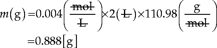
11.

You want to prepare a standard for atomic absorption spectroscopy measurements containing 1000 ppm Ca. How much CaCl₂ do you need to weigh out for 1000 mL stock solution? The atomic mass unit of Ca is 40.078, and the molecular weight of CaCl₂ is 110.98 g/mol.
12.

Outline how you would prepare 250 mL of 0.1 M acetate buffer at pH 5.5 for enzymatic glucose analysis.
13.

Complexometric determination of calcium requires an ammonium buffer with 16.9 g ammonium chloride (molecular weight, 53.49) in 143 mL concentrated ammonium hydroxide solution (28 % wt/wt, density = 0.88; molecular weight = 17; pK_b = 4.74). It is also to contain 1.179 g of Na₂EDTA^.2H₂O (molecular weight = 372.24 g/mol) and 780 mg MgSO₄ ^.7H₂O (molecular weight = 246.47 g/mol).After combining all reagents, the volume is brought up to 250 mL. What are the molarities for EDTA and MgSO₄, and what pH does this buffer have?
14.
Your lab uses 0.2 M stock solutions of NaH₂PO₄ and Na₂HPO₄ for buffer preparation.
1. (a)
  
  Calculate the amounts weighed out for preparing 0.5 L of fresh 0.2 M stock solutions of NaH₂PO₄ ^.H₂O (molecular weight, 138) and Na₂HPO₄ ^.7H₂O (molecular weight, 268).
2. (b)
  
  You want to make 200 mL of a 0.1 M buffer with pH 6.2 from these stock solutions. How many mL of each stock solution do you have to take?
3. (c)
  
  How would the pH change if 1 mL of a 6 M NaOH solution was added (note: you may ignore the volume change)?
15.

Tris (2-amino-2-hydroxymethyl-propane-1,3-diol) is an amino compound suitable for preparation of buffers in physiological pH ranges such as for the dietary fiber assay; however, its pK_a is highly affected by temperature. The reported pKa at 25 °C is 8.06 [3]. Assuming a decline in pK_a of approximately 0.023 ΔpH/°C, what pH would a Tris buffer with a molar acid/base ratio of 4:1 have at 60 °C versus at 25 °C?
16.

Ammonium formate buffers are useful for LC-MS experiments. How would you prepare 1 L of a 0.01 M buffer of pH 3.5 with formic acid (pK_a = 3.75, 98 % wt/wt, density = 1.2) and ammonium formate (molecular weight 63.06 g/mol)? Note: You may ignore the contribution of ammonium ions to the pH and focus on the ratio of formic acid/formate anion. You may treat the formic acid as pure for the calculation, i.e., ignore the % wt/wt.

Prev Next